Simulation of electric vehicle movement
This example will demonstrate the simulation of the movement of an electric vehicle.
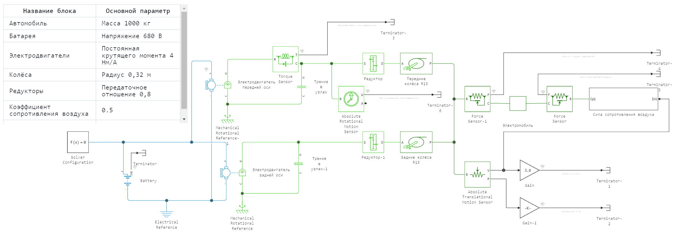
The movement of an electric vehicle and its inertia are described by the block Electric vehicle. The resulting force from two pairs of wheels connected to gearboxes and electric motors that convert and generate torque comes to the left port of this unit. The air resistance force described by the subsystem of the same name is applied to the right port.
The main parameters of the model:
| Block name | The main parameter |
|---|---|
| Car | Weight 1000 kg |
| Battery | Voltage 680 V |
| Electric motors | Torque constant 4 Nm/A |
| Wheels | Radius 0.32 m |
| Gearboxes | Gear ratio 0.8 |
| Air resistance coefficient | 0.5 |
Model diagram:
Defining the function to load and run the model:
function start_model_engee()
    try
        engee.close("electro_car", force=true) # closing the model
        catch err # if there is no model to close and engee.close() is not executed, it will be loaded after catch.
            m = engee.load("$(@__DIR__)/electro_car.engee") # loading the model
        end;

    try
        engee.run(m) # launching the model
        catch err # if the model is not loaded and engee.run() is not executed, the bottom two lines after catch will be executed.
            m = engee.load("$(@__DIR__)/electro_car.engee") # loading the model
            engee.run(m) # launching the model
        end
end
Running the simulation
try
    start_model_engee() # running the simulation using the special function implemented above
    catch err
    end;
Recording speed, torque, and force signals from simout to variables:
t = simout["electro_car/Speed in km/h"].time[:] # time
T = simout["electro_car/Electric motor torque"].value[:] # electric motor torque
speed = simout["electro_car/Speed in km/h"].value[:] # vehicle speed
forces_left = simout["electro_car/Power from the transmission side"].value[:] # forces,
forces_right = simout["electro_car/Air resistance force"].value[:]
w = simout["electro_car/Motor speed"].value[:];
using Plots
Visualization of simulation results
plot(t, forces_left, label="Force from the transmission, N", linewidth=2)
plot!(t, forces_right, label="Air resistance, N", linewidth=2)
plot!(t, (forces_left+forces_right), label="The sum of forces, N", linewidth=2)
After analyzing the "Sum of Forces" curve, you can see that it becomes zero as the forces acting on the electric vehicle are balanced. The movement becomes uniform, with a constant speed.
plot(t, T, label="Electric motor torque, NM", linewidth=2)
plot!(t, (w * 9.55), label="Electric motor rotation speed, rpm", linewidth=2)
plot!(t, (T .* w ./1000), label="Electric motor power, kW", linewidth=2)
As the car accelerates, the torque decreases and the rotation speed of the electric motor increases. The mechanical power produced by this electric motor increases as the force of air resistance increases, depending on the speed.
plot(t, speed, label="Speed, km/h", linewidth=2)
Definition of a function for calculating acceleration time to 100 km/h and its application to electric vehicle speed data:
function acceleration_time(speeds, t)
    # We find the index of the first element exceeding 100 km/h
    index = findfirst(x -> x > 100, speeds)

    # If the index is found, we return the appropriate time.
    if index != nothing
        return println("Acceleration time up to 100 km/h: ", t[index], " with")
    else
        return println("The car did not accelerate to 100 km/h, maximum speed: ", maximum(speed), " km/h")
    end
end

acceleration_time(speed, t)
println("Maximum speed: ", maximum(speed), " km/h")
Conclusion:
This example demonstrates the simulation of the movement of an electric vehicle. He accelerates to a certain steady speed, but the force of air resistance does not allow him to accelerate further. The acceleration time to 100 km/h and the maximum speed of the electric vehicle were calculated.