Simulation of an unstable multivibrator
This example will demonstrate the simulation of an unstable multivibrator.
An unstable multivibrator is a self—oscillating circuit that generates continuous rectangular pulses. It has no stable states and automatically switches between two transistors, creating a periodic signal.
Multivibrators can be used to generate clock signals in various systems.
Mathematical description
The duration of the pulses and pauses is determined by the RC circuits in the base circuits of the transistors.
The duration of the "ON" state for each transistor:
Total oscillation period (with symmetrical scheme):
Frequency of signals:
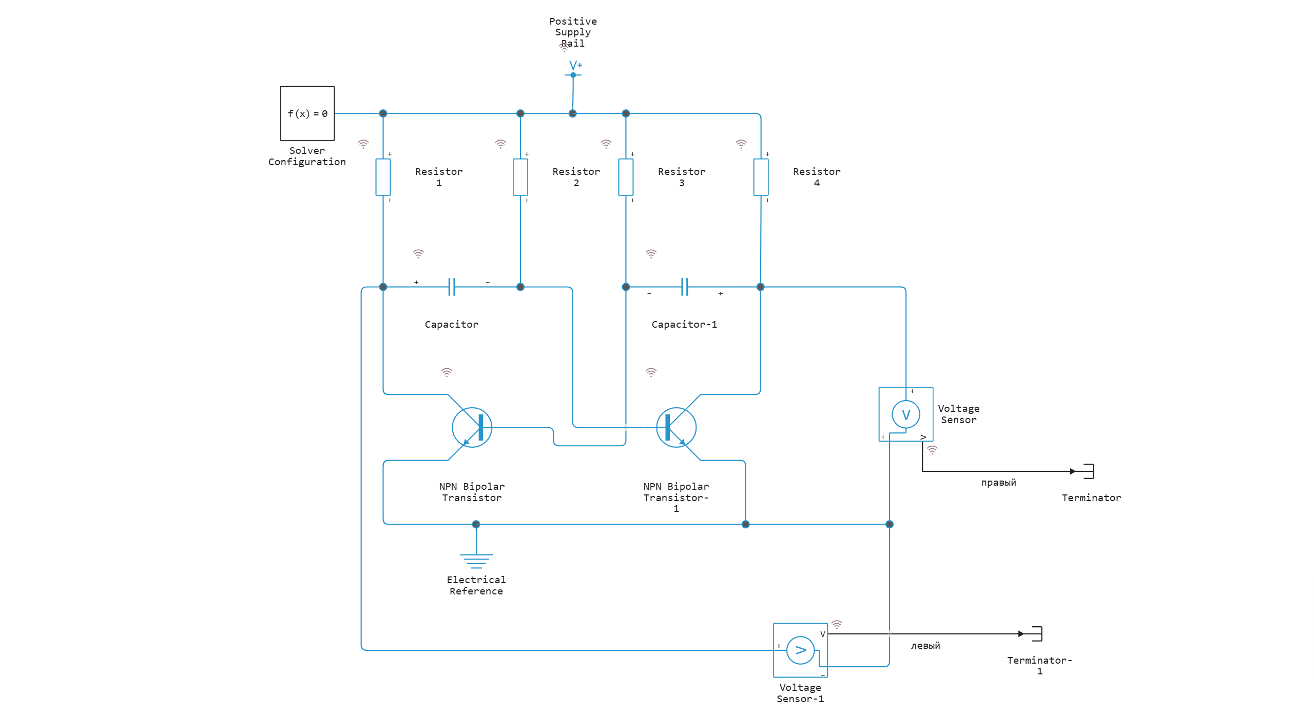
Model diagram:
Defining the function to load and run the model:
function start_model_engee()
    try
        engee.close("npn_transistor", force=true) # closing the model
        catch err # if there is no model to close and engee.close() is not executed, it will be loaded after catch.
            m = engee.load("$(@__DIR__)/astable_multivibrator.engee") # loading the model
        end;

    try
        engee.run(m, verbose=true) # launching the model
        catch err # if the model is not loaded and engee.run() is not executed, the bottom two lines after catch will be executed.
            m = engee.load("$(@__DIR__)/astable_multivibrator.engee") # loading the model
            engee.run(m, verbose=true) # launching the model
        end
end
Running the simulation
start_model_engee();
Writing simulation data to variables:
t = simout["astable_multivibrator/right"].time[:]
V_right = simout["astable_multivibrator/right"].value[:]
V_left = simout["astable_multivibrator/left"].value[:]
I_R1 = simout["Resistor 1.i"].value[:]
I_R4 = simout["Resistor 4.i"].value[:]
Data visualization
using Plots
Visualization of collector-emitter voltage on both transistors:
plot(t, V_left, linewidth=2)
plot!(t, V_right, linewidth=2)
Visualization of current on resistors connected to transistor collectors:
plot(t, I_R1, linewidth=2)
plot!(t, I_R4, linewidth=2)
Processing simulation results:
Launching the statistics library:
using Statistics
Definition of a function for finding the frequency and period of voltage fluctuations:
function calculate_oscillation_properties(time::Vector{T}, x::Vector{T}) where T <: Real
    # Checking the length of vectors
    if length(time) != length(x)
        error("The time and signal vectors must be the same length.")
    end
    n = length(time)
    n < 2 && return (NaN, NaN)  # Insufficient data

    # We find the average value of the signal
    avg = sum(x) / n

    # We are looking for the points of intersection of the average value from bottom to top
    up_crossings = T[]
    for i in 2:n
        if x[i-1] < avg && x[i] >= avg
            # Linear interpolation to accurately determine the time of intersection
            t = time[i-1] + (time[i] - time[i-1]) * (avg - x[i-1]) / (x[i] - x[i-1])
            push!(up_crossings, t)
        end
    end

    # Checking for a sufficient number of intersections
    length(up_crossings) < 2 && return (NaN, NaN)

    # Calculation of periods (in time units)
    periods = diff(up_crossings)
    mean_period = mean(periods)
    frequency = 1 / mean_period

    return "Oscillation frequency: $frequency Hz. Fluctuation period: $mean_period with."
end
Applying a function to a vector of voltage values (any signals can be substituted):
calculate_oscillation_properties(collect(t)[:,1], collect(V_left)[:,1])
Conclusions:
In this example, we have considered a model of an unstable multivibrator, where the key elements determining the frequency and period of oscillation are the base resistors (R2, R3) and capacitors forming time-lapse RC circuits. Collector resistors (R1, R4) have no effect on the frequency of the signal — their role is limited to limiting the current through the transistors and forming the amplitude of the output voltage.