Simulation of a bipolar PNP transistor
This example will demonstrate the simulation of a bipolar transistor at different values of the base current.
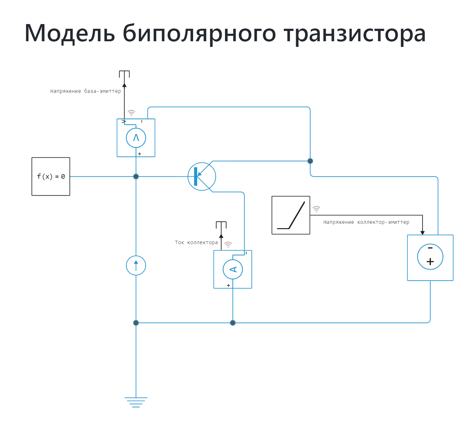
General view of the model:
Defining a function to load and run the model:
In [ ]:
function start_model_engee()
    try
        engee.close("pnp_transistor", force=true) # closing the model
        catch err # if there is no model to close and engee.close() is not executed, it will be loaded after catch.
            m = engee.load("/user/start/examples/physmod/pnp_transistor/pnp_transistor.engee") # loading the model
        end;

    try
        engee.run(m, verbose=true) # launching the model
        catch err # if the model is not loaded and engee.run() is not executed, the bottom two lines after catch will be executed.
            m = engee.load("/user/start/examples/physmod/pnp_transistor/pnp_transistor.engee") # loading the model
            engee.run(m, verbose=true) # launching the model
        end
end
Out[0]:
Loading, running the model, and recording the results
Simulation at a base current of -0.001 A:
In [ ]:
Ib = -0.001 # determining the base current for calculation
start_model_engee() # loading and launching the model
sleep(5)
data1 = collect(simout) # extracting data from the simout variable describing collector current and collector-emitter voltage
Vce = collect(data1[1]) # recording collector-emitter voltage data in a variable
Ic1 = collect(data1[2]); # recording collector current data in a variable
Simulation with a base current of -0.002 A:
In [ ]:
Ib = -0.002 # determining the base current for calculation
start_model_engee() # loading and launching the model
sleep(5)
data2 = collect(simout) # extracting data from the simout variable describing collector current and collector-emitter voltage
Ic2 = collect(data2[2]); # recording collector current data in a variable
Simulation with a base current of -0.003 A:
In [ ]:
Ib = -0.003 # determining the base current for calculation
start_model_engee() # loading and launching the model
sleep(5)
data3 = collect(simout) # extracting data from the simout variable describing collector current and collector-emitter voltage
Ic3 = collect(data3[2]); # recording collector current data in a variable
Simulation with a base current of -0.004 A:
In [ ]:
Ib = -0.004 # determining the base current for calculation
start_model_engee() # loading and launching the model
sleep(5)
data4 = collect(simout) # extracting data from the simout variable describing collector current and collector-emitter voltage
Ic4 = collect(data4[2]); # recording collector current data in a variable
Simulation with a base current of -0.005 A:
In [ ]:
Ib = -0.005 # determining the base current for calculation
start_model_engee() # loading and launching the model
sleep(5)
data5 = collect(simout) # extracting data from the simout variable describing collector current and collector-emitter voltage
Ic5 = collect(data5[2]); # recording collector current data in a variable
Visualization of results
In [ ]:
using Plots # launching the charting library:
plot(Vce[:,2], Ic1[:,2], label="Base current, Ib = -0.001 A", title="Graph of the dependence of collector current on collector-emitter voltage")
plot!(Vce[:,2], Ic2[:,2], label="Base current, Ib = -0.002 A", xlabel="Vce, In", ylabel="Ic, And")
plot!(Vce[:,2], Ic3[:,2], label="Base current, Ib = -0.003 A")
plot!(Vce[:,2], Ic4[:,2], label="Base current, Ib = -0.004 A")
plot!(Vce[:,2], Ic5[:,2], label="Base current, Ib = -0.005 A")
Out[0]:
Conclusion:
In this example, a simulation of a bipolar transistor was demonstrated at different values of the base current. The model can also be used to determine the characteristics of a transistor in the positive voltage range ().