Simulation of a malfunction of an armature winding of an electric motor
This example simulates the operation of a DC motor with an armature winding malfunction.
Model diagram:
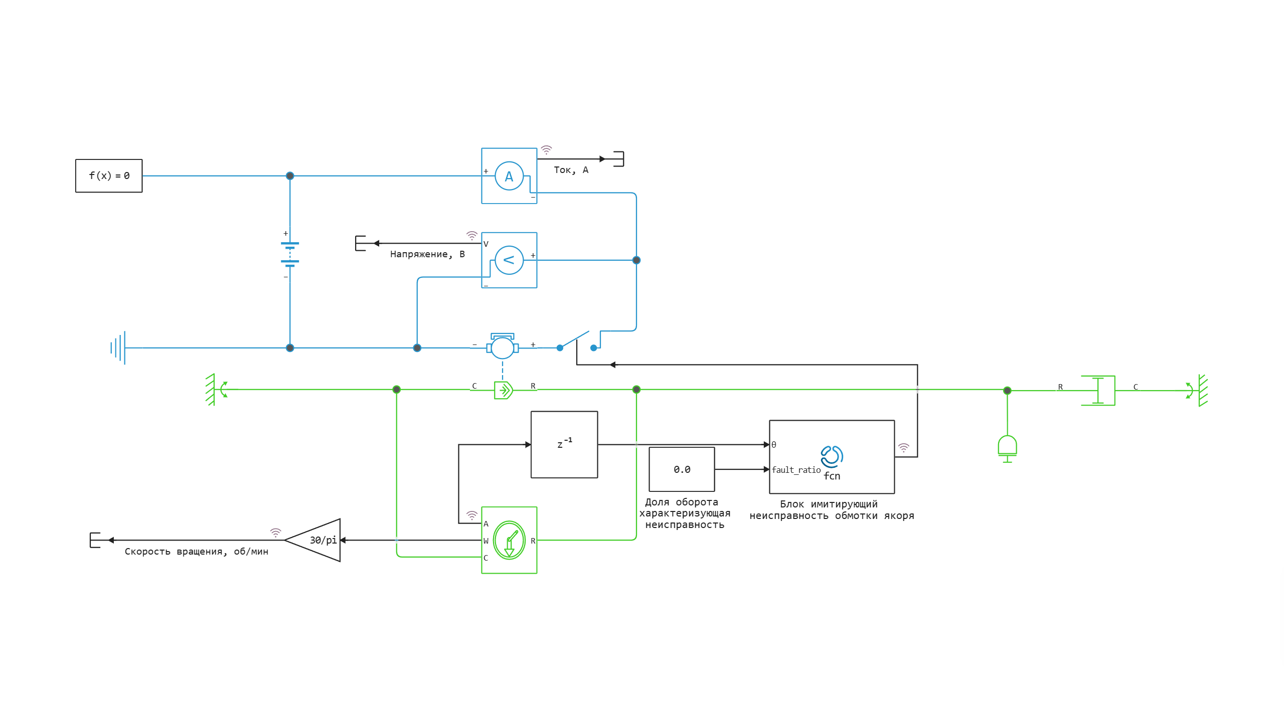
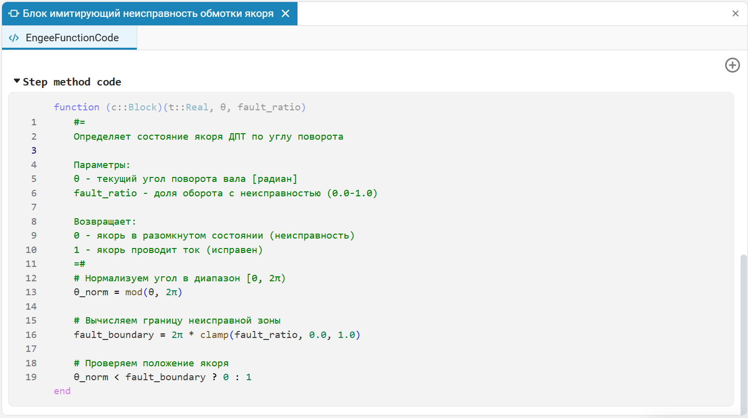
A malfunction of the armature winding of a DC motor is simulated using the Engee Function block, in which, in the Step method code section, a function in the Julia programming language is built in. The function takes two arguments, the angle of rotation and the fraction of a revolution with a malfunction, and returns signals 1 or 0, which characterize a serviceable or faulty condition, respectively.
The signal from the Engee Function unit enters the Key unit, opening and closing the motor armature circuit.
Defining the function to load and run the model:
function start_model_engee()
    try
        engee.close("simple_motor_armature_winding_fault", force=true) # closing the model
        catch err # if there is no model to close and engee.close() is not executed, it will be loaded after catch.
            m = engee.load("$(@__DIR__)/simple_motor_armature_winding_fault.engee") # loading the model
        end;

    try
        engee.run(m) # launching the model
        catch err # if the model is not loaded and engee.run() is not executed, the bottom two lines after catch will be executed.
            m = engee.load("$(@__DIR__)/simple_motor_armature_winding_fault.engee") # loading the model
            engee.run(m) # launching the model
        end
end
Running the simulation
Simulation without malfunction:
start_model_engee();
Isolation of rotation speed, current and voltage signals from the simout variable:
result = simout;
res1 = collect(result)
Malfunction of the armature winding:
engee.set_param!("simple_motor_armature_winding_fault/Доля оборота
 characterizing
 неисправность", "Value" => 0.0833)
Starting a simulation with an armature winding malfunction:
engee.run("simple_motor_armature_winding_fault");
Isolation of rotation speed, current and voltage signals from the simout variable:
result = simout;
res2 = collect(result)
Writing signals to variables:
w_1 = collect(res1[2])
w_2 = collect(res2[2]);
Visualization of simulation results
Graph of the motor speed without malfunction and with malfunction of the armature winding:
using Plots
Plots.plot(w_1[:,1], w_1[:,2], label="Rotation speed of a serviceable DPT, rpm", linewidth=3)
Plots.plot!(w_2[:,1], w_2[:,2], label="Rotation speed of the faulty DPT, rpm", linewidth=2)
It can be seen that the steady rotation speed has become lower with the introduction of the malfunction.
Plots.plot(w_1[:,1], w_1[:,2], label="Rotation speed of a serviceable DPT, rpm", linewidth=3)
Plots.plot!(w_2[:,1], w_2[:,2], label="Rotation speed of the faulty DPT, rpm", linewidth=2, xlim=(6.15, 6.50), ylim=(3400, 3700))
By zooming in on the graph, you can see an unstable engine speed with an armature winding malfunction.
Conclusions:
Analysis of the simulation results shows that the DC motor reaches a stable rotational speed close to the nominal value (at rated load) within a few seconds after starting; when the fault is activated in steady state, the speed decreases to a new stable value, less than the initial value.