The model of movement of a car with a CVT
A detailed physico-mathematical model of car dynamics is presented. Its key task is to study the complex interaction of the power unit, transmission, chassis and roadway in transitional and steady—state modes, starting from engine start.
The model is focused on solving the following engineering tasks: analyzing the effect of transmission parameters on acceleration dynamics and fuel efficiency, the effect of imperfect traction in the longitudinal direction, and optimizing control algorithms (simulating the operation of a variator).
Feature: The model focuses on the start and initial acceleration stages, where the role of the torque converter and differentials is critically important, and also allows you to observe steady motion.
demoroot = @__DIR__
mdl = engee.open(joinpath(demoroot,"vehicle_simple_4wheel.engee"))
Description of the model
Model type vehicle_simple_4wheel.engee:
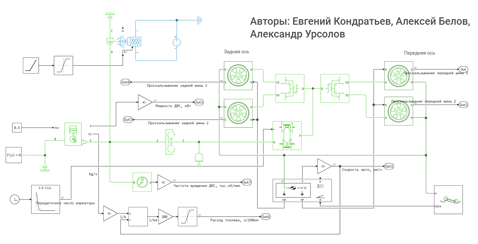
Key physical blocks:
-
Roadbed (RoadProfile): Sets the vertical profile for calculating normal reactions and effects on the suspension. It is used to generate basic traffic scenarios.
-
Body and suspension (Vehicle Body): It takes into account the vertical dynamics through the suspension models of the front and rear axles. Calculates the normal reactions transmitted to the tire model.
-
Startup and initial acceleration (MotorAndDrive+ GenericEngine):
-
The start process is initiated by The basic starter/electric drive model (MotorAndDrive), which applies an initial torque to the motor shaft.
-
After starting, the engine (GenericEngine) operates according to the static characteristic (torque map), without complex control algorithms. Its main function is to generate torque depending on the throttle position and calculate the conditional fuel consumption.
-
Important: Control signals (throttle, transmission restriction) are implemented by directional signals (for example, Step, Signal Builder) for simplicity and clarity
-
-
Transmission is the heart of the model (GDT, CVT, Differentials):
-
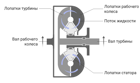
Torque Converter (GDT): provides a smooth start and demonstrates a low-speed slip mode.
-
Variator: A gearbox that dynamically transmits motion and torque between the two connected axes of the drive shafts: the driving and the driven.
-
Differentials: The gear mechanism, which allows the driven gears to rotate at different speeds, simulates the kinematics of the axes. Viscous friction can be set in them.
-
-
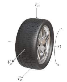
Tires and wheels: convert torque into traction force, taking into account slippage. At the start stage, under equal conditions, the wheel slippage of one axle is identical.
Simulation of the model
When running the model in the "Signal Visualization" window, you can see all the logged signals depending on the simulation time, namely:
- Car speed, km/h
- Slipping of all tires
- Internal combustion engine power, kW
- Engine rotation speed, thousand rpm
- CVT gear ratio
- Fuel consumption, l/100 km
Saving simulation results to the workspace:
result = engee.run(mdl);
Let's unpack some of the recorded signals with the function collect:
vehicle_speed = collect(result["Car speed, km/h"]);
engine_power = collect(result["Internal combustion engine power, kW"]);
slip_front_1 = collect(result["Front tire slip 1"]);
slip_front_2 = collect(result["Front tire slip 2"]);
slip_rear_1 = collect(result["Rear tire slip 1"]);
slip_rear_2 = collect(result["Rear tire slip 2"]);
Let's display on the graph the dependence of the internal combustion engine power on time.:
plot(engine_power.time,engine_power.value,lw=3,label="engine_power",
            title = "Internal combustion engine power from time to time",
            xguide = "Time (s)",
            yguide = "Power, kW")
We will also display on the graph the slippage of four tires at the initial moment of the simulation (up to 2.5 seconds):
plot(slip_front_1.time,slip_front_1.value,l=:steppost, label="slip_front_1")
plot!(slip_front_2.time,slip_front_2.value,l=:steppost, label="slip_front_2")
plot!(slip_rear_2.time,slip_rear_2.value,l=:steppost, label="slip_rear_2")
plot!(slip_rear_1.time,slip_rear_1.value,l=:steppost, label="slip_rear_1",
        xlim = (0,2.5),
        title = "Tire slippage",
        xguide = "Time (s)")
A similar difference is observed due to the fact that the Front Tire block 1 has an imperfection - longitudinal stiffness and damping are taken into account.
It is also worth noting the possibility of taking into account advanced physical phenomena in all blocks modeling the components of the vehicle.
Conclusion
We have considered a model that can be used as a starting point for building a virtual stand, which, in turn, will allow engineers to analyze complex cross-effects in the driver-car-road system, focusing on the dynamics of start and steady motion.