Parameterization of an asynchronous motor with a closed rotor
In this example, using the passport data of an asynchronous motor with a closed-loop rotor, we calculate and simulate an asynchronous motor from the "Electricity" section of the block library.
Introduction
An example of parameterization of an asynchronous motor (AD) with a closed-loop rotor (KZR) was given earlier for constructing a vector диаграммы. Here is a slightly improved code with the passport data of another engine. Subsequent modeling in Engee is performed using the block Asynchronous machine with a short circuit ротором from the Electricity section of the [Physical Modeling] Block library(https://engee.com/helpcenter/stable/en/getting-started-physmod.html ).
Initial data
For an example of calculation and simulation, let's take the AIR132 S4 engine with a rotation speed of 1455 rpm. His passport details are easy to find on the Internet. Let's write them into the corresponding variables of the code cell below.:
Pₙ = 7.5e3; Uₙ = 380; f₁ = 50;           # Rated power [W], line voltage [V], frequency [V]
nₙ = 1455; p = 2; η = 0.87;              # Rated rotation speed [rpm], number of pole pairs, efficiency
cosϕ = 0.83; Iₙ = 15.8;       # Rated power factor, rated current [A], no-load current [A]
ki = 7; mₚ = 2.3; mₘ = 2.3; J = 0.02;   # Coefficients of maximum current, starting and maximum torque, moment of inertia of the motor [kg·m2]
We will make intermediate calculations:
# Calculation of substitution scheme parameters
U₁ = Uₙ/sqrt(3);                           # Rated phase voltage of the stator [V]
n₀ = 60*f₁/p;                             # Synchronous rotation speed [rpm]
sₙ = (n₀-nₙ)/n₀; sₖ = sₙ*(mₘ+sqrt(mₘ^2-1)); # Nominal and critical slip
ω₀ = 2π*f₁/p; ωₙ = π*nₙ/30;                # Synchronous and nominal angular velocity of the rotor [rad/s]
Mₙ = Pₙ/ωₙ; Mₘ = Mₙ*mₘ; Mₚ = Mₙ*mₚ;           # Nominal, maximum and starting torque [Nm]
pₘ = 0.05*Pₙ;                              # Mechanical losses (5% of Pₙ) [W]

R₂ = 1/3*(Pₙ+pₘ)/(Iₙ^2*(1-sₙ)/sₙ);              # The reduced active resistance of the rotor winding is [Ohms]

C = 1.02;                   # Constructive coefficient (preliminary)

R₁ = U₁*cosϕ*(1-η)/Iₙ - C^2*R₂ - pₘ/(3*Iₙ^2);  # Active resistance of the stator winding [Ohms]

L₁σ = L₂σ = U₁/(4π*f₁*(1+C^2)*ki*Iₙ);          # Stator dissipation inductance and reduced rotor [Gn]
L₁ = L₂ = U₁/(2π*f₁*Iₙ*sqrt(1-cosϕ^2)-2/3*(2π*f₁*Mₘ*sₙ)/(p*U₁*sₖ)); # Stator inductance and reduced rotor [Gn]
Lₘ = L₁ - L₁σ;                                 # Magnetic circuit inductance [Gn]
Let's perform several iterations to refine the design coefficient.:
for i in 1:5

    C = 1 + L₁σ/Lₘ                             # Constructive coefficient (specified)

    R₁ = U₁*cosϕ*(1-η)/Iₙ - C^2*R₂ - pₘ/(3*Iₙ^2);  # Active resistance of the stator winding [Ohms]

    L₁σ = L₂σ = U₁/(4π*f₁*(1+C^2)*ki*Iₙ);          # Stator dissipation inductance and reduced rotor [Gn]
    L₁ = L₂ = U₁/(2π*f₁*Iₙ*sqrt(1-cosϕ^2)-2/3*(2π*f₁*Mₘ*sₙ)/(p*U₁*sₖ)); # Stator inductance and reduced rotor [Gn]
    Lₘ = L₁ - L₁σ;                                 # Magnetic circuit inductance [Gn]

    println("Iteration #$i: The refined constructive coefficient C is equal to $C")
end

    X₁σ = 2π*f₁*L₁σ;    X₂σ = 2π*f₁*L₂σ        # Reactive resistances of stator dissipation and reduced rotor [Ohms]
    Xₘ = 2π*f₁*Lₘ;
All the necessary parameters for modeling the ADCZR in Engee have been calculated, let's move on to modeling.
The network, load, and engine parameters defined above are also written in reverse вызовах example models. This allows you to run the model with the "default" parameters without first calculating them.
The example model
The example model is a simple chain with a KZR control unit - the motor is connected directly to the network, the ends of the stator winding are connected to a "star", the mechanical load is represented by a source of torque and a moment of inertia.
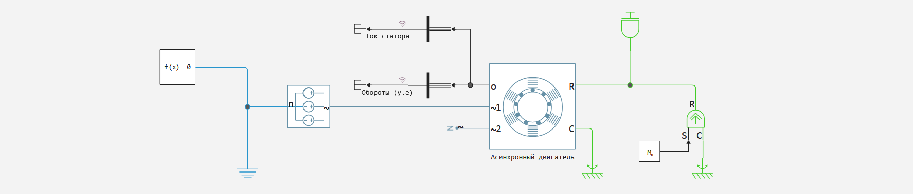
Let's run the model using software modeling control and pre-prepared functions for ease of working with the model and simulation results:
example_path = @__DIR__; # We get the absolute path to the directory containing the current script
cd(example_path); # Go to the example directory
include("useful_functions.jl"); # We connect the Julia script with auxiliary functions
simout = get_sim_results("im_parametrization.engee", example_path) # running the simulation
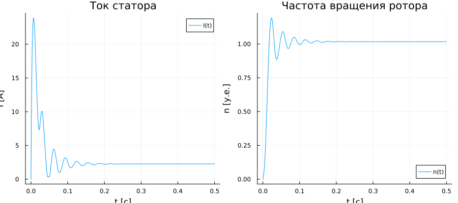
We get the variables of the signals recorded in the model:
t = get_sim_data(simout, "Stator current", 1, "time");
Is = get_sim_data(simout, "Stator current", 1, "value");
n = get_sim_data(simout, "Revolutions (units)", 1, "value");
Let's plot these variables:
gr(aspectratio=:auto, xlims=:auto, ylims=:auto, size = (900,400))
I_graph = plot(t, Is; label = "I(t)", title = "Stator current", ylabel = "I [A]", xlabel = "t [s]")
n_graph = plot(t, n; label = "n(t)", title = "Rotor speed", ylabel = "n [units]", xlabel = "t [s]")
plot(I_graph, n_graph)
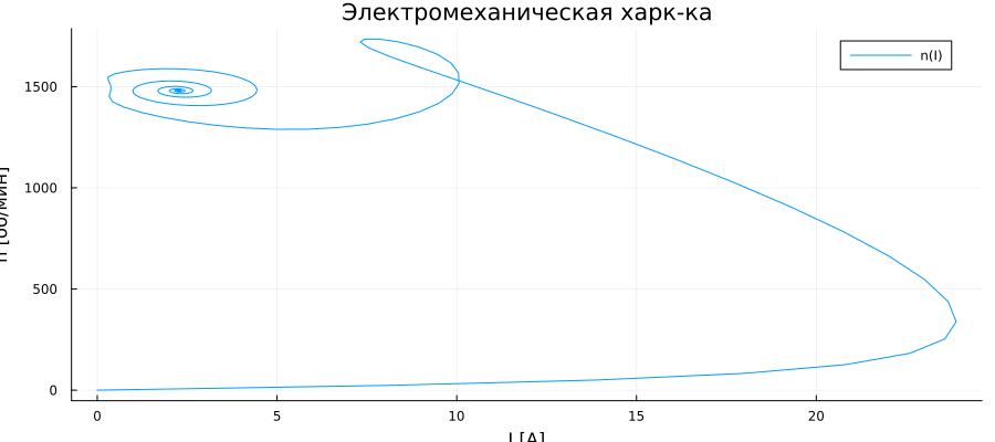
In conclusion, we will construct an electromechanical characteristic:
gr(aspectratio=:auto, xlims=:auto, ylims=:auto, size = (900, 400))
plot(Is, n.*nₙ; label = "n(I)", title = "Electromechanical hark-ka", ylabel = "n [rpm]", xlabel = "I [A]")
Conclusion
In the example, we looked at an example of parameterizing an asynchronous motor model based on passport data from open sources, conducting BP modeling and data collection. Next, you can proceed to the development of an engine control system or simulation of a technological unit with this engine.