Pressure drop and mass flow rate in the heat-conducting liquid pipeline
In this example, we will study how friction and height differences affect the pressure drop in the pipe, as well as how accounting for the dynamic compressibility of the liquid will affect the mass flow through the pipe. These effects are especially important in long and narrow pipes, since in such systems it is necessary to set an increased flow pressure to compensate for losses.
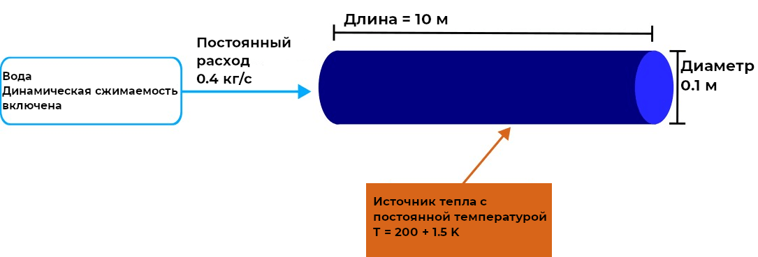
Consider a 10-meter-long pipeline with a circular cross-section with a diameter of 0.1 m. The mass flow rate in the pipe is constant and amounts to 0.4 kg/s. The water comes from the tank at a temperature of 293.15 K and under atmospheric pressure. The effects of dynamic compressibility of a liquid were not initially taken into account.
We will set the mass flow rate, length and diameter of the pipe.
mdot = 0.4;       # [kg/s] Mass consumption
pipe_length = 10; # [m] Pipe length
D = 0.1;          # [m] Pipe diameter
Pressure drop due to height difference
How will the model of this pipe behave if the height difference between its entrance and exit is 3 meters? Let's ignore the effect of friction and calculate the pressure drop analytically, and then use the model to verify the result.
.png)
Pressure drop in a pipe is the sum of pressure losses due to friction against the pipe walls and due to height differences.
where - pressure drop due to height change in the pipe, — pressure drop due to friction against the pipe walls. Since we neglect friction, we can assume equal to zero and use to define using the Bernoulli equation.
The Bergulli equation relates the velocity, pressure, and height of a fluid at different points in a hydrodynamic system, and we use it to calculate the properties of the fluid at points A and B of the pipe model:
where — pressure at point A or B, — density of the liquid, — the flow rate at point A or B, — acceleration of free fall, — the height of the liquid at point A or B.
When modeling an incompressible fluid, the mass is preserved and , where - consumption at point A, — flow rate at point B.
Flow rate is the product of the density, velocity, and cross—sectional area of the pipe. If we assume that the density of the liquid and the cross-sectional area of the pipe are constant along its entire length, then due to the conservation of flow and conservation of momentum can be used by equality due to this , the terms with this variable on both sides of the Bernoulli equation can be eliminated and the expression can be shortened to:
where — height difference between points A and B.
Let's perform an analytical calculation of the expected pressure loss due to the height difference. You can change the height difference in the model by changing the variable delta_z:
delta_z = 3;     # [m] Height difference
g = 9.81;        # [m/s^2] Acceleration of gravity
rho = 998;       # [kg/m3] Water density at 293.15 K and 101325 Pa

deltaP_h = rho*g*delta_z   # [Pa] Analytical calculation of pressure drop due to height difference
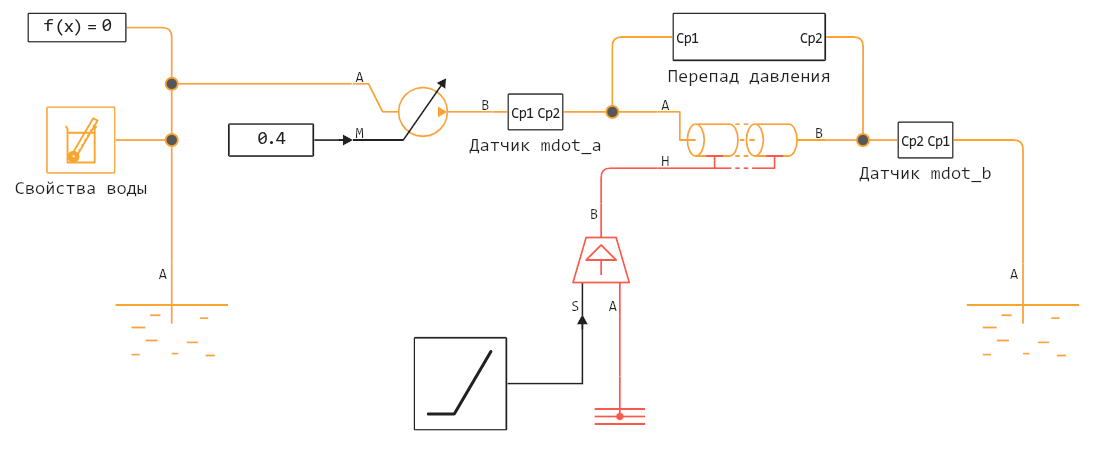
Now let's run the model PressureLossAndFlowRateInTLPipe_Insulated, which allows you to calculate the outflow of a constant flow through a pipe between two tanks, pumped by a pump providing a constant flow rate of 0.4 kg/s.
# engee.close_all()
model = engee.open("$(@__DIR__)/PressureLossAndFlowRateInTLPipe_Insulated.engee")
delta_z = 3;
engee.run(model);
Let's build a graph and study the calculation results.:
t = pressure_drop.time;
delta_P = pressure_drop.value;
plot( t, delta_P, ylimits = (2.93e4,2.94e4),
      xlabel="Time, from", ylabel="Pressure drop, 10⁴ Pa",
      yformatter = x->"$(x/10000)", legend=false, lw=2 )
It is impossible to completely remove the friction in the Pipe block, so the results include friction losses, but they are significantly less than the loss due to the height difference. The results show a constant pressure loss of about Pa, which is consistent with the analytical results (* error of three hundredths of a percent*).
Pressure loss due to friction
Friction losses are usually much less than losses due to height differences. However, if the height difference is If it is equal to zero, friction losses will be the main cause of pressure loss in the pipe.
Consider a brass pipe in which the surface roughness of the inner wall is M. Let's perform an analytical calculation of pressure losses due to friction in the pipe, and then check the Engee model for consistency with the results.
.png)
Pressure losses due to friction primarily depend on the Reynolds number of the fluid. The Reynolds number is a dimensionless quantity used in hydrodynamics to predict the flow pattern. It represents the ratio of inertia of a liquid to its viscosity. At low Reynolds numbers, the liquid tends to have a rather laminar flow (inertia far exceeds viscosity), and as the Reynolds number increases, the flow becomes more turbulent.
The Reynolds number is usually expressed as follows:
where:
-
— flow rate,
-
— dynamic viscosity of the liquid,
-
— pipe diameter.
Using the expression for expense you can rewrite the expression:
where — the cross-sectional area of the pipe.
Calculate the Reynolds number for the water in the pipe:
S = pi/4 * D^2;      # [m^2] Pipe cross-sectional area
mu = 0.00102;        # [Pa*s] Dynamic viscosity of water at 293 K and 0.101325 MPa

Re = mdot*D/(S*mu)   # the Reynolds number
A flow having a Reynolds number of more than 4000 is usually considered turbulent, that is, a flow in which chaotic changes in pressure and velocity play a significant role. The pressure loss due to friction in a turbulent regime is expressed by the following equation:
where — pipe length, — Darcy's coefficient of friction.
The Darcy coefficient of friction is a dimensionless quantity describing the frictional resistance in a pipe. Friction resistance is a force that prevents the movement of liquid relative to the inner surface of the pipe. Friction slows down the flow, which leads to a drop in pressure, which can be expressed by the following formula:
where — a measure of the absolute roughness of the inner surface.
epsilon = 1.52e-6;    # [m] Absolute roughness of the inner surface for commercial brass, lead, copper or plastic pipes

f = 1 / (-1.8 * log10(6.9/Re + (epsilon/3.7)^1.11))^2;          # The Darcy coefficient of friction
deltaP_f = f * pipe_length * mdot * abs(mdot) / (2*rho*D*S^2)   # [Pa] Pressure loss due to friction
Let's launch the model PressureLossAndFlowRateInTLPipe_Insulatedmodel and check the amount of pressure loss due to friction.
model = engee.open("$(@__DIR__)/PressureLossAndFlowRateInTLPipe_Insulated.engee")
delta_z = 0;       # [m] Pipe height
engee.run(model);
Let's plot the results and study them.
t = pressure_drop.time;
delta_P = pressure_drop.value;
plot( t, delta_P, ylimits = (4.85,4.95),
      xlabel="Time, from", ylabel="Pressure drop, 10⁴ Pa",
      legend=false, lw=2 )
The model shows a constant pressure drop of 4.878 Pa, which corresponds to the analytical result of 4.905 Pa (error of about half a percent).
We can evaluate the effect of the pipe wall material with different friction loss coefficients on pressure loss.:
Material  = ["Brass/Lead/Copper/Plastic", "Steel or iron (forged)", "Cast iron", "Cast iron and rust"];
Roughness = [1.52e-6, 4.6e-5, 2.59e-4, 1.5e-3]; # [m] Absolute roughness of the inner surface

f         = 1 ./ (-1.8 .* log10.(6.9/Re .+ (Roughness./3.7).^1.11)).^2;    # The Darcy coefficient of friction
Pressure_Loss  = f .* pipe_length .* mdot .* abs(mdot) ./ (2*rho*D*S^2);   # [Pa] Pressure drop due to friction
using DataFrames
T = DataFrame("Material" => Material, "Roughness" => Roughness, "Pressure drop" => Pressure_Loss)
The table shows how the pressure drop depends on the material and condition of the pipe. The differences are small, but in sensitive systems they lead to relatively large energy losses.
Conservation of mass and compressibility of liquid
Now let's explore how the flow rate in the pipe will be affected by taking into account the effect of dynamic compressibility and adding a heat source to the model.
If you disable the "Dynamic compressibility" parameter (Fluid dynamic compressibility), the pipeline model will not take into account the dynamic effects in the mass of liquid inside the pipe and the outlet flow rate will always be equal to the inlet flow rate.:
where - flow rate through the cross section A, - flow rate through the section B.
Since the model considered so far is designed exactly like this, the flow rate at both ends of the pipe will be the same.
model = engee.open("$(@__DIR__)/PressureLossAndFlowRateInTLPipe_Insulated.engee")
delta_z = 0;       # [m] Pipe height
engee.run(model);
Here are the calculation results for the model without taking into account compressibility.
t = pressure_drop.time;
mdot_a_incompressible = mdot_a.value;
mdot_b_incompressible = mdot_b.value;
plot( t, [mdot_a_incompressible -mdot_b_incompressible],
      xlabel="Time, from", ylabel="Mass flow rate, (kg/s)", lw=2,
      ls=[:solid :dash], label=["mdot_a" "- mdot_b"], ylimits=(-0.5,0.5) )
The mass flow rate in ports A and B is equal in magnitude and opposite in sign.
This behavior can change if the dynamic compressibility of the fluid is enabled. Since the mass of the compressible fluid is unevenly distributed along the entire length of the pipe, the mass balance equation includes additional terms:
where:
-
— the volume of liquid in the pipe,
-
— density,
-
— pressure,
-
— temperature,
-
— isothermal modulus of volumetric elasticity,
-
— isobaric coefficient of thermal expansion.
Because the pipe is perfectly insulated and the pressure loss due to friction is negligible., and . Both values can be ignored. In this case, since the right-hand side of the mass balance equation is still approximately zero, the pipe behaves the same as in the case of an incompressible medium, and the mass flow rate between port A and port B does not change.
Let's turn on the dynamic compressibility of the liquid in the Pipeline block:
engee.set_param!( "PressureLossAndFlowRateInTLPipe_Insulated/Pipe (Advanced) (TL)",
   "dynamic_compressibility" => true )
Let's run the model and plot the graphs:
engee.run(model);

t = pressure_drop.time;
mdot_a_compressible = mdot_a.value;
mdot_b_compressible = mdot_b.value;
plot( t, [mdot_a_compressible -mdot_b_compressible],
      xlabel="Time, from", ylabel="Mass flow rate, (kg/s)", lw=2,
      ls=[:solid :dash], label=["mdot_a" "- mdot_b"], ylimits=(-0.5,0.5) )
The mass expenses in ports A and B are still equal in magnitude and opposite in sign.
To observe a significant difference in consumption, we will add heat transfer accounting by connecting a heat source to the model. Then the component of the equation containing the term it will reach a noticeable size. Consider a model in which the temperature of a heat source connected to a pipe varies linearly over time.
.png)
.png)
Let's plot the temperature in the presence of a heat source in the model.
t = 0:0.1:120
temperature = 200 .+ 1.5t;
plot( t, temperature, xlabel="Time (s)", ylabel="Temperature (K)")
The inclusion of the heat transfer effect in the model leads to the fact that the right-hand side of the mass balance equation becomes quite noticeable, and the mass flow rate at the outlet of the pipe begins to increase. Open and runPressureLossAndFlowRateInTLPipe_HeatSource.
model = engee.open("$(@__DIR__)/PressureLossAndFlowRateInTLPipe_HeatSource.engee");
engee.set_param!( "PressureLossAndFlowRateInTLPipe_HeatSource/Pipe (Advanced) (TL)",
   "dynamic_compressibility" => true )
engee.run(model);
And let's build a graph with the results.
t = pressure_drop.time;
mdot_a_compressible = mdot_a.value;
mdot_b_compressible = mdot_b.value;
plot( t, [mdot_a_compressible -mdot_b_compressible],
      xlabel="Time, from", ylabel="Mass flow rate, (kg/s)", lw=2,
      ls=[:solid :dash], label=["mdot_a" "- mdot_b"], ylimits=(0.39,0.41) )
Conclusion
At the beginning of the simulation, the source temperature was 200 K, which is less than the water temperature in the pipe, which is 293.15 K. After 55 seconds have elapsed, the temperature of the heat source has exceeded the temperature of the water flowing into the pipe. In the first half of the experiment, the rate of temperature change in the pipe was negative, meaning that . After the temperature of the heat source has exceeded the temperature of the water entering the pipe, heat begins to be transferred to the pipe. In this case, the rate of temperature change has become positive, which leads to .