Modelling of pipeline pressure control

This example demonstrates the modelling of pressure control in a pipeline.

Working principle of the model

The pipeline is described by blocks of the physical modelling library, in particular, the Volume block is responsible for its volume.

Through Valve 1 the liquid flows from Source to Volume. This in turn is connected to a Pressure sensor, from which the signal is fed to the control system represented by an adder, a setpoint adjuster and a PID controller.

Schematic diagram of the model:

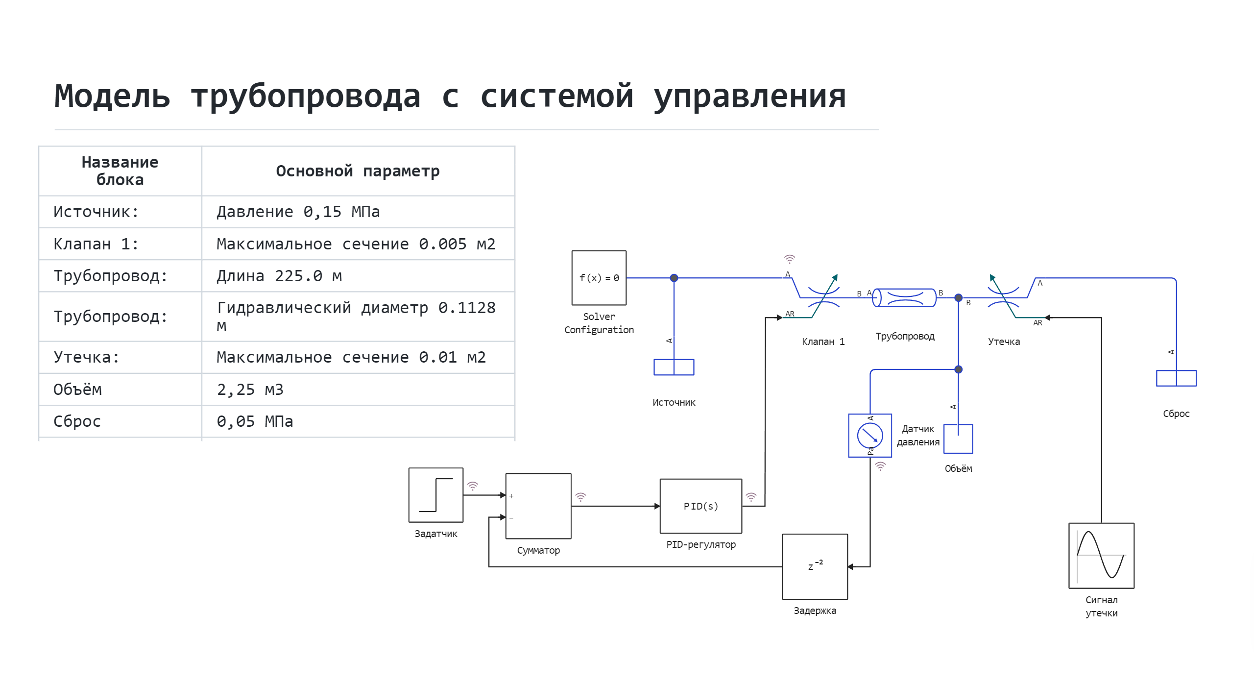
The PID controller sends a control signal to Valve 1 to open or close, providing pressure regulation.

To the right of the Volume block, in the fluid path, is the Leak block, which is, like Valve 1, a controlled throttle.

The Leak block creates some "random" fluid flow from the simulated pipeline.

The fluid passing through this block eventually enters the Discharge, which is described by an infinite reservoir with a given pressure.

Boundary conditions

1. At the source, the pressure is always maintained at 151.3 kPa.
2. In the reservoir, which characterises the space where the liquid is discharged through a leak, the pressure is always 50 kPa.

Initial conditions:

1. The initial pressure in the pipeline is 100 kPa.
2. The setpoint signal is 100000, which in the context of regulation means 100 kPa.

Define the function to load and run the model:

function start_model_engee()
    try
        engee.close("liquid_pressure_regulator", force=true) # закрытие модели 
        catch err # в случае, если нет модели, которую нужно закрыть и engee.close() не выполняется, то будет выполнена её загрузка после catch
            m = engee.load("$(@__DIR__)/liquid_pressure_regulator.engee") # загрузка модели
        end;

    try
        engee.run(m) # запуск модели
        catch err # в случае, если модель не загружена и engee.run() не выполняется, то будут выполнены две нижние строки после catch
            m = engee.load("$(@__DIR__)/liquid_pressure_regulator.engee") # загрузка модели
            engee.run(m) # запуск модели
        end
end

start_model_engee (generic function with 1 method)

Running the simulation

try
    start_model_engee() # запуск симуляции с помощью специальной функции, реализованной выше
    catch err
    end;

Selecting the temperature data of the plots from the simout variable and writing them to variables:

sleep(5)
result = simout;
res = collect(result)

28-element Vector{WorkspaceArray}:
 WorkspaceArray("liquid_pressure_regulator/Step.1")
 WorkspaceArray("liquid_pressure_regulator/Клапан 1.port_a.p")
 WorkspaceArray("liquid_pressure_regulator/Утечка.rho_b")
 WorkspaceArray("liquid_pressure_regulator/Утечка.Vdot_b")
 WorkspaceArray("liquid_pressure_regulator/Утечка.restriction_area_in.u")
 WorkspaceArray("liquid_pressure_regulator/Клапан 1.rho_a")
 WorkspaceArray("liquid_pressure_regulator/Add.1")
 WorkspaceArray("liquid_pressure_regulator/Утечка.mdot_b")
 WorkspaceArray("liquid_pressure_regulator/Утечка.port_b.p")
 WorkspaceArray("liquid_pressure_regulator/Утечка.Vdot_a")
 WorkspaceArray("liquid_pressure_regulator/Клапан 1.port_b.mdot")
 WorkspaceArray("liquid_pressure_regulator/Клапан 1.mdot_a")
 WorkspaceArray("liquid_pressure_regulator/Клапан 1.restriction_area_in.u")
 ⋮
 WorkspaceArray("liquid_pressure_regulator/PID Controller.1")
 WorkspaceArray("liquid_pressure_regulator/Клапан 1.Vdot_a")
 WorkspaceArray("liquid_pressure_regulator/Клапан 1.port_b.p")
 WorkspaceArray("liquid_pressure_regulator/Утечка.delta_p")
 WorkspaceArray("liquid_pressure_regulator/Утечка.mdot_a")
 WorkspaceArray("liquid_pressure_regulator/Утечка.rho_a")
 WorkspaceArray("liquid_pressure_regulator/Клапан 1.mdot_b")
 WorkspaceArray("liquid_pressure_regulator/Утечка.port_a.mdot")
 WorkspaceArray("liquid_pressure_regulator/Датчик давления.1")
 WorkspaceArray("liquid_pressure_regulator/Утечка.port_a.p")
 WorkspaceArray("liquid_pressure_regulator/Утечка.port_b.mdot")
 WorkspaceArray("liquid_pressure_regulator/Клапан 1.Vdot_b")

Writing the setpoint and pressure sensor signals to variables:

control_signal = collect(res[1])
pressure = collect(res[25])

10,001 rows × 2 columns

	time	value
	Float64	Float64
1	0.0	100000.0
2	0.01	1.00048e5
3	0.02	1.00097e5
4	0.03	1.00145e5
5	0.04	1.00132e5
6	0.05	100176.0
7	0.06	1.00164e5
8	0.07	1.00166e5
9	0.08	1.00155e5
10	0.09	1.00144e5
11	0.1	100134.0
12	0.11	1.00123e5
13	0.12	1.00113e5
14	0.13	1.00103e5
15	0.14	1.00092e5
16	0.15	1.00082e5
17	0.16	1.00072e5
18	0.17	1.00061e5
19	0.18	1.00051e5
20	0.19	1.00041e5
21	0.2	1.00031e5
22	0.21	1.00022e5
23	0.22	1.00012e5
24	0.23	1.00002e5
25	0.24	99992.2
26	0.25	99982.6
27	0.26	99973.0
28	0.27	99963.5
29	0.28	99954.0
30	0.29	99944.6
⋮	⋮	⋮

Visualisation of simulation results

using Plots
plot(control_signal[:,1], control_signal[:,2], label="Задатчик", linewidth=3)
plot!(pressure[:,1], pressure[:,2], label="Датчик давления", linewidth=3)

Conclusion:

In this example, modelling of a physical object with an automatic control system has been demonstrated. The transient time is about 15 s, the pressure stabilises within acceptable limits, its minor fluctuations are related to the leakage of liquid from the pipeline.

Blocks used in example

• Pipe (IL)
• Absolute Pressure Sensor (IL)
• Delay
• Sine Wave Function
• Step