Simulation of a solenoid with a return spring
This script will demonstrate a simulation of a solenoid with a return spring.
When the power is turned off, the spring pulls the piston 5 mm away from the center of the coil. Turning on the power supply at t =0.1 s draws the piston into the center of the coil. At t=0.3 s, an external load of 10 N. is applied to the plunger.
The solenoid is modeled here using blocks from a library of magnetic components.
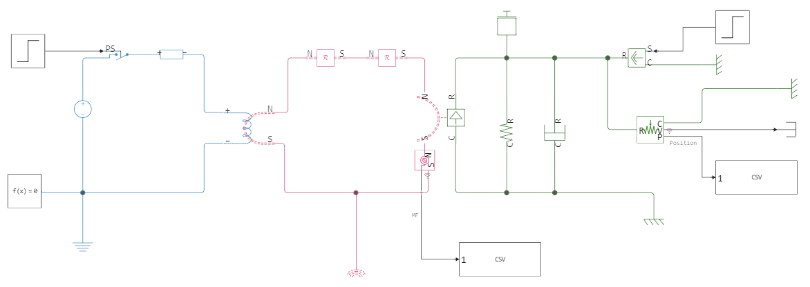
The principle of operation:
The current passing through the solenoid creates a magnetomotive force that creates a flow through the magnetic core of the solenoid. A counteracting force is created, which actuates the piston, which closes the air gap, initially having a length of 5 mm. The flow in the magnetic circuit increases as the length of the air gap decreases.
Implementation of the model launch using software control:
Loading the model:
modelName = "Solenoid_with_Magnetic_Blocks";
actuator_model = modelName in [m.name for m in engee.get_all_models()] ? engee.open( modelName ) : engee.load( "$(@__DIR__)/$(modelName).engee");
Launching the uploaded model:
results = engee.run( modelName );
Loading and visualizing the data obtained during the simulation.
Reading csv files with data on the movement of the solenoid and on changes in the magnetic flux,
followed by conversion into a dataframe and matrix.
position = results["Position"];
MF = results["MF"];
Connecting the library for charting:
using Plots
Enabling a backend graphics display method:
gr()
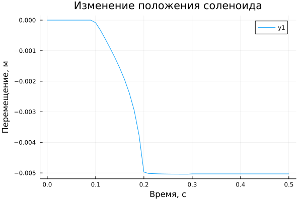
Plotting a graph describing the change in the position of the solenoid.
plot(position.time, position.value, xlabel="Time, from", ylabel="Displacement, m", title="Changing the position of the solenoid")
Plotting a graph describing the change in magnetic flux.
plot(MF.time, MF.value, xlabel="Time, from", ylabel="Magnetic flux, Wb", title="Changing the magnetic flux")
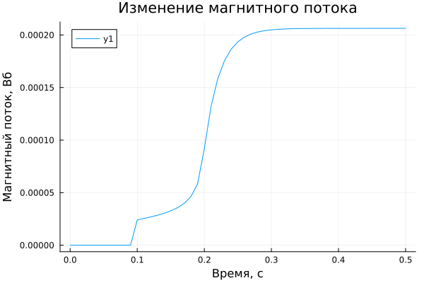
Conclusion
In this example, it was demonstrated that as the solenoid moves and the air gap decreases, the value of the magnetic flux increases.