Differential paired amplifier
This example will demonstrate the simulation of a differential paired amplifier.
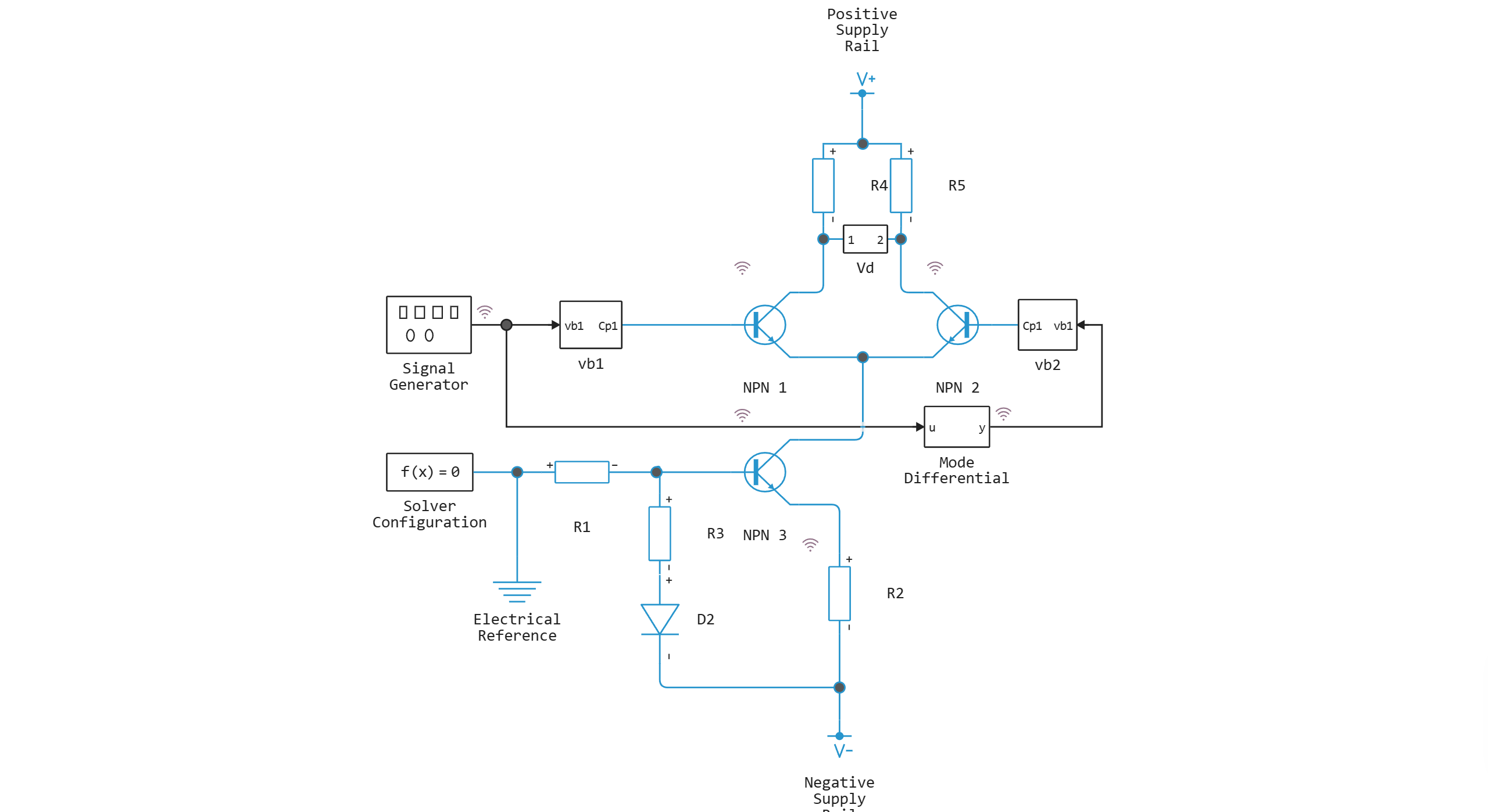
Model diagram:
Defining the function to load and run the model:
In [ ]:
function start_model_engee()
    try
        engee.close("differential_pair_amplifier", force=true) # closing the model
        catch err # if there is no model to close and engee.close() is not executed, it will be loaded after catch.
            m = engee.load("$(@__DIR__)/differential_pair_amplifier.engee") # loading the model
        end;

    try
        engee.run(m, verbose=true) # launching the model
        catch err # if the model is not loaded and engee.run() is not executed, the bottom two lines after catch will be executed.
            m = engee.load("$(@__DIR__)/differential_pair_amplifier.engee") # loading the model
            engee.run(m, verbose=true) # launching the model
        end
end
Out[0]:
Running the simulation
In [ ]:
start_model_engee();
Writing simulation data to variables:
In [ ]:
t = simout["differential_pair_amplifier/Signal Generator.1"].time[:]
vb1 = simout["differential_pair_amplifier/Signal Generator.1"].value[:]
vb2 = simout["differential_pair_amplifier/Mode Differential.y"].value[:]
vc1 = simout["differential_pair_amplifier/Vd/Voltage Sensor p.1"].value[:]
vc2 = simout["differential_pair_amplifier/Vd/Voltage Sensor n.1"].value[:]
vc2_minus_vc1 = simout["differential_pair_amplifier/Vd/Voltage Sensor d.1"].value[:]
vb2_minus_vb1 = vb2 .- vb1;
Data visualization
In [ ]:
using Plots
Visualization of voltage on collectors of NPN 1 and NPN2 transistors:
In [ ]:
plot(t, vb1, linewidth=2, label="vb1")
plot!(t, vb2, linewidth=2, label="vb2")
plot!(t, vb2_minus_vb1, linewidth=2, label="vb2-vb1", title="Input voltage")
Out[0]:
In [ ]:
plot(t, vc1, linewidth=2, label="vc1")
plot!(t, vc2, linewidth=2, label="vc2")
plot!(t, vc2_minus_vc1, linewidth=2, label="vc2-vc1", title="Output voltage")
Out[0]:
Conclusions:
In this example, we have considered the model of a differential paired amplifier. The graphs show the output and input characteristics of the amplifier, which differ by more than 40 times.