Temperature measurement during steel quenching
This example shows how using the "Thermocouple" unit allows you to simulate measuring the temperature of steel during quenching.
During quenching, the steel is heated to a temperature above the recrystallization temperature, and then quickly cooled by immersion in liquid. Due to the high temperature, it is impossible to use traditional temperature measuring instruments (thermistor or semiconductor temperature sensors, liquid thermometers). To measure temperatures in such harsh conditions, industry and laboratories use thermocouples that convert thermal potential differences into electrical potential differences.
Model Overview
Open the model thermocouple_quenching.
cd(@__DIR__) # Go to the folder with the example
engee.open("thermocouple_quenching.engee");
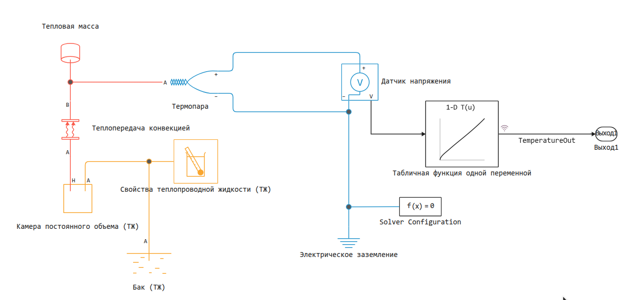
In this model, the "Thermal Mass" block simulates a steel cylinder heated to an initial temperature of 850°C. The "Constant Volume Chamber" block simulates a quenching bath and cools the cylinder to 20°C by forced convection.
Calculation and output of graphs
In this calculation experiment, we will change the parameters of different blocks. Just in case, we'll set the initial parameters again, with which we get the first results.
engee.set_param!("thermocouple_quenching/Термопара", "parameterization"=>"Type K (t≥0 degC)")
engee.set_param!("thermocouple_quenching/Термопара", "C_vector"=>"TypeK_Cvec")
engee.set_param!("thermocouple_quenching/Табличная функция одной переменной",
"Table"=>"TypeK_degC", "BreakpointsForDimension1"=>"TypeK_Volts")
engee.set_param!("thermocouple_quenching/Теплопередача конвекцией",
"h" => Dict("value" => 4000, "unit" => "W/(m^2*K)"))
Let's execute the model:
data = engee.run("thermocouple_quenching")
plot(data["TemperatureOut"].time, data["TemperatureOut"].value, leg=false, lw=2)
The "1-D search table" block connects the output voltage of the "Thermocouple" block to the temperature scale, that is, it allows you to convert volts to degrees. Let's output a logarithmic graph of the time dependence of the temperature of the thermocouple and the temperature of the cylinder and make sure that the calculated and actual values match.
tempOut = data["TemperatureOut"]
tempCylinder = data["Thermal mass.T"]
plot( tempOut.time, tempOut.value, xaxis = (:log10, [10^-1, :auto]), lw=2 )
plot!( tempCylinder.time, tempCylinder.value .- 273.15, c=:red, ls=:dash, lw=2 )
As we can see, after converting to degrees Celsius, the graphs match very well.
Let's see how the temperature of the liquid in the tank changed.
tempVolume = data["A constant volume camera (TJ).T"]
plot( tempVolume.time, tempVolume.value .- 273.15,
xaxis = (:log10, [10^-1, :auto]), lw=2, ls=:dashdot, leg=false )
The model of the properties of a thermally conductive liquid is limited by maximum temperatures, therefore, in order to avoid overheating, sufficiently large values of the volume of the cooling tank and the volume of the interface between the tank and the environment (the "Tank" block) are prescribed in the model.
We see that the liquid reaches a temperature of 52.1°C (325.3K), remaining within the permissible limits set by the following values:
maxTemp = engee.get_param("thermocouple_quenching/Свойства теплопроводной жидкости (ТЖ)", "T_max_2D");
minTemp = engee.get_param("thermocouple_quenching/Свойства теплопроводной жидкости (ТЖ)", "T_min_2D");
println("Maximum allowable temperature: ", maxTemp["value"], maxTemp["unit"])
println("Minimum allowable temperature: ", minTemp["value"], minTemp["unit"])
Change to type S thermocouple (TPP10)
Currently, the parameters of the "Thermocouple" unit correspond to a type K thermocouple (TCA), and the nonlinear characteristic for this unit is available in the NIST ITS-90 database[1]. We'll save the results for later comparison.:
TypeK_tout = tempOut;
TypeK_vout = data["Thermocouple.p.v"];
To calculate the type S thermocouple (TPP10). Let's switch our thermocouple unit to another mode.:
engee.set_param!("thermocouple_quenching/Термопара", "parameterization"=>"Type B, E, J, K (t≤0 degC), N, R, S or T")
We will substitute the available coefficients for the type S thermocouple as the coefficients of the thermocouple model.:
engee.set_param!("thermocouple_quenching/Термопара", "C_vector"=>"TypeS_Cvec")
In addition, we will change the table in the nonlinear correction block ("Tabular function of one variable") to the appropriate ones.:
engee.set_param!("thermocouple_quenching/Табличная функция одной переменной",
"Table"=>"TypeS_degC", "BreakpointsForDimension1"=>"TypeS_Volts")
Let's run this model and also save the results for comparison.:
data = engee.run("thermocouple_quenching")
plot(data["TemperatureOut"].time, data["TemperatureOut"].value, leg=false, lw=2)
TypeS_tout = data["TemperatureOut"];
TypeS_vout = data["Thermocouple.p.v"];
Now we can deduce the output characteristics of both types of thermocouples.:
plot( TypeS_vout.time, TypeS_vout.value, xaxis = (:log10, [10^-1, :auto]), ls=:dashdot, lw=2, label="Type S" )
plot!( TypeK_vout.time, TypeK_vout.value, c=:red, ls=:dash, lw=2, label="Type K" )
The voltage at the positive output of different types of thermocouples is different. But the temperature measurements calculated at the output are the same.
plot( TypeS_tout.time, TypeS_tout.value, xaxis = (:log10, [10^-1, :auto]), ls=:dashdot, lw=2, label="Type S" )
plot!( TypeK_tout.time, TypeK_tout.value, c=:red, ls=:dash, lw=2, label="Type K" )
Changing heat transfer properties
In this example, the parameter "Coefficient of specific heat capacity" of the "Thermal mass" block and the "Coefficient of heat transfer" of the "Heat transfer by convection" block are estimates obtained in a laboratory study of a scale model of industrial hardening of a steel cylinder in water[2].
For simplicity, these parameters are set as constants. For more accurate results, it would be necessary to set them as a function of temperature (if data is available), but there is an easier way. You can run simulations with different values of these parameters and get a range of estimates.
Set the parameter "Heat transfer coefficient" in the "Heat transfer by convection" block to 4000.
engee.set_param!("thermocouple_quenching/Теплопередача конвекцией",
"h" => Dict("value" => 2000, "unit" => "W/(m^2*K)"))
Let's run the model and build a graph.
data = engee.run("thermocouple_quenching")

tempOut4000 = TypeK_tout;
tempOut2000 = data["TemperatureOut"]
plot( tempOut2000.time, tempOut2000.value, ls=:dash, lw=2, label="2000 W/(K*m)^2" )
plot!( tempOut4000.time, tempOut4000.value, c=:red, xaxis = (:log10, [10^-1, :auto]), lw=2, label="4000 W/(K*m)^2", ls=:dashdot )
Conclusion
This model is designed to accurately measure the temperature of steel during quenching using a thermocouple, where conventional sensors do not work. To improve the result, you need to use real dependences of the heat transfer coefficient on temperature, rather than constant values.
Bibliography
[1] Angela Y. Lee, NIST ITS-90 Thermocouple Database - SRD 60, National Institute of Standards and Technology, 2000. https://data.nist.gov/od/id/ECBCC1C1302A2ED9E04306570681B10748.
[2] Hasan, H. S., M. J. Peet, J. M. Jalil, and H. K. D. H. Bhadeshia. “Heat Transfer Coefficients during Quenching of Steels.” Heat and Mass Transfer 47, no. 3 (March 2011): 315–21. https://doi.org/10.1007/s00231-010-0721-4.