Investigation of torsional oscillations of a multi-mass system
This example will show the modeling and analysis of torsional vibrations of a multi-mass mechanical system. The model demonstrates how an impulse action excites the system's own modes, and how a resonant effect leads to a significant amplification of vibrations.
Torsional vibrations occur in systems with several inertial masses connected by elastic shafts. Each such system has a set of natural frequencies (modes) at which resonant amplification of vibrations occurs.
Initial excitation: a pulse moment of 1000 Nm with a duration of 0.01 s.
Model diagram:
To implement the torsional vibration model, a multi-mass system with elastic bonds is used.
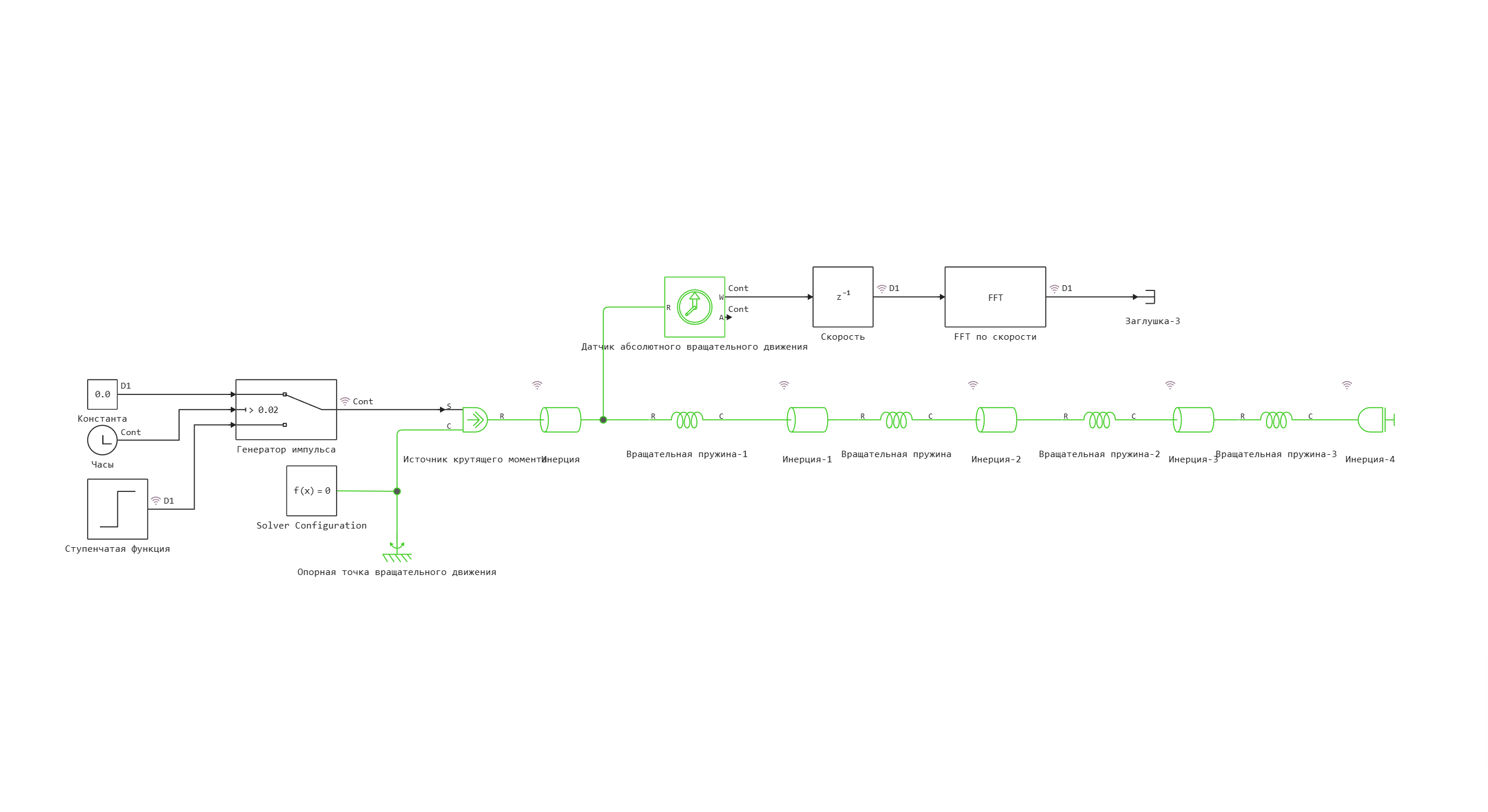
Defining the function to load and run the model:
m = "torsional_oscillations"
function start_model_engee(m)
    try
        engee.close(m, force=true) # closing the model if it is open
    catch err # in case there is no model to close.
        # The model was not opened
    end

    try
        m = engee.load("$((@__DIR__))/$m.engee") # loading the model
        engee.run(m) # launching the model
    catch err # in case the model is not loaded
        m = engee.load("$((@__DIR__))/$m.engee") # loading the model
        engee.run(m) # launching the model
    end
end
Defining functions for analysis:
Natural frequency analysis FFT function:
import Pkg;
Pkg.add(["DSP", "Peaks"])
using FFTW, DSP

function analyze_natural_frequencies(time_data, speed_data)
    # Preparing data for FFT
    dt = time_data[2] - time_data[1]
    fs = 1/dt  # Sampling rate

    # Applying the window function for better resolution
    windowed_data = speed_data .* hanning(length(speed_data))

    # FFT Calculation
    fft_result = fft(windowed_data)

    # Frequency axis
    frequencies = fftfreq(length(fft_result), fs)

    # Amplitude spectrum in dB
    magnitude_db = 20 * log10.(abs.(fft_result) .+ 1e-10)

    return frequencies, magnitude_db
end
Natural frequency peak search function:
using Peaks

function find_natural_frequencies(frequencies, magnitude_db, min_height=20)
    # Search for peaks in the positive part of the spectrum
    pos_freq_idx = frequencies .> 0
    pos_freqs = frequencies[pos_freq_idx]
    pos_magnitudes = magnitude_db[pos_freq_idx]

    # Search for local maxima
    peaks, _ = findmaxima(pos_magnitudes)

    # Height filtering
    high_peaks = peaks[pos_magnitudes[peaks] .> min_height]

    natural_freqs = pos_freqs[high_peaks]
    amplitudes = pos_magnitudes[high_peaks]

    return natural_freqs, amplitudes
end
Starting a simulation with a pulse effect
start_model_engee(m);
By running the model in the simulation environment, in the Signal Visualization window, you can see a graph of the velocity signal after the FFT (fast Fourier transform) in the frequency domain.:
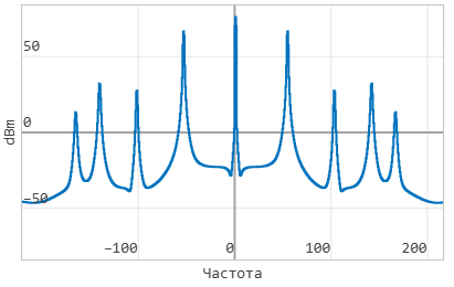
By analyzing this graph, it is possible to detect the natural frequencies of the system.
Let's build a similar graph in this interactive script. To do this, output the simulation data to variables.
Output of data for analysis:
# Obtaining the angular velocities of all inertia
omega1 = collect(simout["torsional_oscillations/FFT by speed.1"]);

# Allocating time and data for analysis
time_data = omega1[:,1];
speed_data = omega1[:,2];  # Analyzing the first inertia
Performing FFT analysis:
# FFT analysis for determining natural frequencies
frequencies, magnitude_db = analyze_natural_frequencies(time_data, speed_data);
natural_freqs, amplitudes = find_natural_frequencies(frequencies, magnitude_db);

# Output of the found natural frequencies
println("Detected natural frequencies:")
for (i, (freq, amp)) in enumerate(zip(natural_freqs, amplitudes))
    println("$(i)-I mode: $(round(freq, digits=2)) Hz ($(round(amp.-30, digits=2)) dBm)")
end
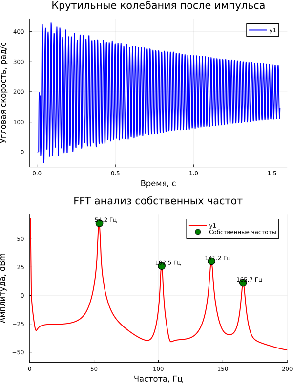
Visualization of the analysis performed:
using Plots
using Printf

function create_torsional_analysis_plots(time_data, speed_data, frequencies, magnitude_db)
    gr()

    # Convert all data to real numbers
    real_frequencies = real.(frequencies)
    real_magnitude_db = real.(magnitude_db)
    real_time_data = real.(time_data)
    real_speed_data = real.(speed_data)

    # Time response schedule
    p1 = plot(real_time_data, real_speed_data,
              title="Torsional vibrations after an impulse",
              xlabel="Time, from",
              ylabel="Angular velocity, rad/s",
              linewidth=2,
              linecolor=:blue)

    # FFT Spectrum graph
    pos_idx = (real_frequencies .> 0) .& (real_frequencies .< 300)
    p2 = plot(real_frequencies[pos_idx], real_magnitude_db[pos_idx] .- 30,
              title="FFT natural frequency analysis",
              xlabel="Frequency, Hz",
              ylabel="Amplitude, dBm",
              xlim=(0, 200),
              linewidth=2,
              linecolor=:red)

    # Allocation of found natural frequencies
    experimental_freqs = natural_freqs
    experimental_amps = amplitudes .- 30

    scatter!(p2, experimental_freqs, experimental_amps,
            markersize=8,
            markercolor=:green,
            markerstroke=:black,
            label="Natural frequencies")

    # Frequency signatures
    for (i, (freq, amp)) in enumerate(zip(experimental_freqs, experimental_amps))
        annotate!(p2, freq+5, amp+3, text(@sprintf("%.1f Hz", freq), 8, :black))
    end

    # Combining graphs
    combined_plot = plot(p1, p2, layout=(2,1), size=(600,800))

    return combined_plot
end

# Creating graphs
analysis_plots = create_torsional_analysis_plots(time_data, speed_data, frequencies, magnitude_db)
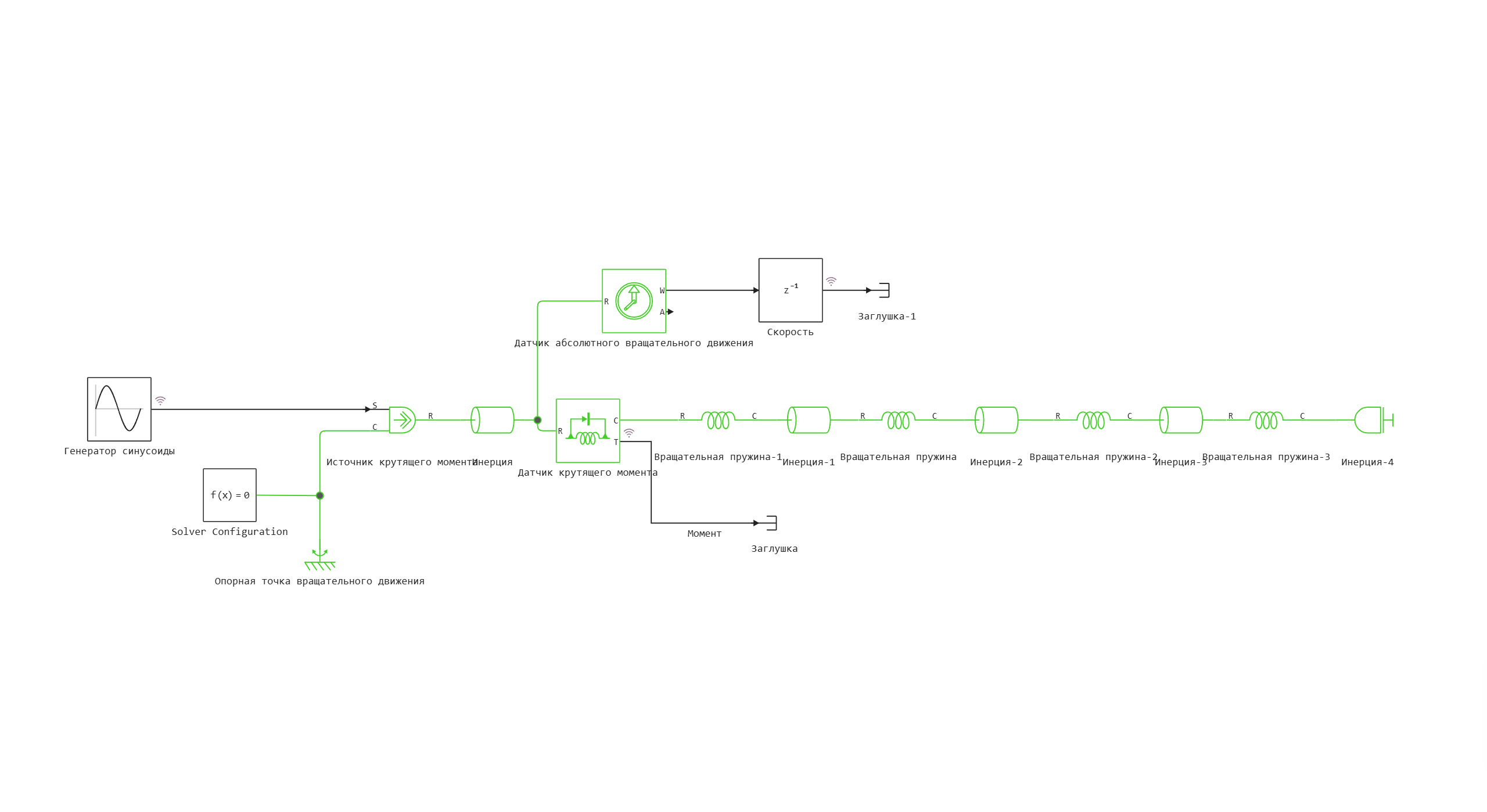
The phenomenon of resonance at natural frequency
Now let's check how the different frequencies of the acting torque source affect the angular velocity of the first inertia block.
The amplitude of the torque is 1 Nm.
To do this, let's run a model where a sinusoidal signal is used as the source of exposure, not a pulse generator.
Model diagram:
Using the variable omega, we determine the frequency of the sinusoidal signal before each simulation run.
n = "torsional_oscillations_sin"
omega = 10
start_model_engee(n)
w = collect(simout["$n/Speed.1"]);
torque = collect(simout["$n/Moment"]);
time_data1 = w[:,1];
speed_data1 = w[:,2];
time_torque = torque[:,1]
torque_data = torque[:,2]
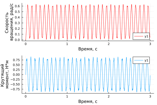
p1 = plot(time_data1, speed_data1, xlabel="Time, from", ylabel="Rotation speed, rad/s", color="red")
p2 = plot(time_torque, torque_data, xlabel="Time, from", ylabel="Torque moment, N*m")
plot(p1,p2, layout=(2,1))
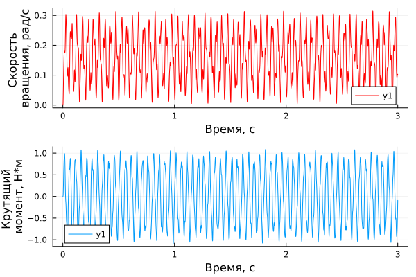
omega = 20
start_model_engee(n)
w = collect(simout["$n/Speed.1"]);
torque = collect(simout["$n/Moment"]);
time_data1 = w[:,1];
speed_data1 = w[:,2];
time_torque = torque[:,1]
torque_data = torque[:,2]
p1 = plot(time_data1, speed_data1, xlabel="Time, from", ylabel="Rotation speed, rad/s", color="red")
p2 = plot(time_torque, torque_data, xlabel="Time, from", ylabel="Torque moment, N*m")
plot(p1,p2, layout=(2,1))
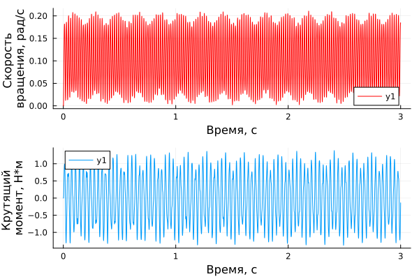
omega = 30
start_model_engee(n)
w = collect(simout["$n/Speed.1"]);
torque = collect(simout["$n/Moment"]);
time_data1 = w[:,1];
speed_data1 = w[:,2];
time_torque = torque[:,1]
torque_data = torque[:,2]
p1 = plot(time_data1, speed_data1, xlabel="Time, from", ylabel="Rotation speed, rad/s", color="red")
p2 = plot(time_torque, torque_data, xlabel="Time, from", ylabel="Torque moment, N*m")
plot(p1,p2, layout=(2,1))
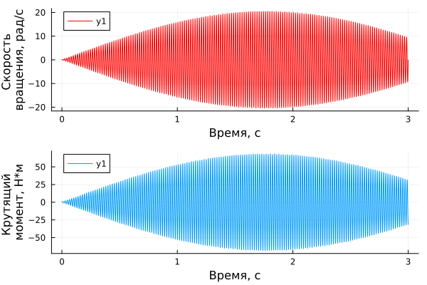
omega = natural_freqs[1] # The first natural frequency
start_model_engee(n)
w = collect(simout["$n/Speed.1"]);
torque = collect(simout["$n/Moment"]);
time_data1 = w[:,1];
speed_data1 = w[:,2];
time_torque = torque[:,1]
torque_data = torque[:,2]
p1 = plot(time_data1, speed_data1, xlabel="Time, from", ylabel="Rotation speed, rad/s", color="red")
p2 = plot(time_torque, torque_data, xlabel="Time, from", ylabel="Torque moment, N*m")
plot(p1,p2, layout=(2,1))
omega = 60
start_model_engee(n)
w = collect(simout["$n/Speed.1"]);
torque = collect(simout["$n/Moment"]);
time_data1 = w[:,1];
speed_data1 = w[:,2];
time_torque = torque[:,1]
torque_data = torque[:,2]
p1 = plot(time_data1, speed_data1, xlabel="Time, from", ylabel="Rotation speed, rad/s", color="red")
p2 = plot(time_torque, torque_data, xlabel="Time, from", ylabel="Torque moment, N*m")
plot(p1,p2, layout=(2,1))
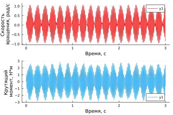
It can be seen that, unlike other frequencies, exposure to natural frequency causes a multiple increase in torque and rotational inertia. The phenomenon of "beating" is observed, which is often accompanied by resonance.
Conclusions:
In this example, a comprehensive model for analyzing torsional vibrations of a multi-mass system was demonstrated.
The model can be adapted for various torsion systems: turbo generator sets, rolling mill drives, marine shaft lines and other industrial mechanisms.