Hydraulic flow rectifier circuit
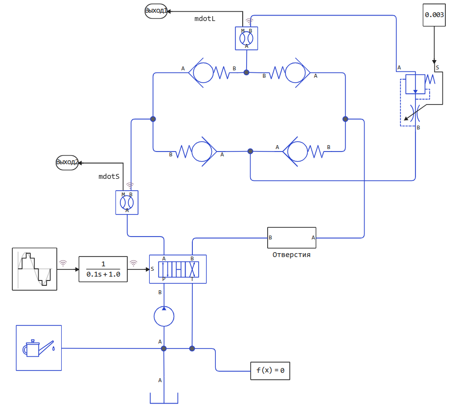
This example shows a flow rectifier circuit with four check valves and one control valve. This scheme allows you to control the flow of liquid from different sources using a single control valve.
The valves are arranged in the same way as the diodes in a diode bridge (Gretz circuit), so the flow always passes through the control valve in the same direction. The "Holes" subsystem contains two more check valves that allow the flow to flow in different directions through holes of different diameters.
Opening the model
Using the Engee software control, we will open the model and examine its device.
cd(@__DIR__) # Go to the folder with the example
engee.open("hydraulic_flow_rectifier.engee");
Because in the block
4-линейный 3-позиционный клапан (ИЖ)there is no dynamic model, we additionally smooth the input signal using a transfer function. It can be considered part of the valve model.Inside all other blocks (
Обратный клапан) the switching dynamics accounting model is enabled. The time constant is 0.01 s.
The "Holes" subsystem looks like this:
.png)
Let's run the model and plot the graphs:
data = engee.run("hydraulic_flow_rectifier")
plot( data["mdotS"].time, [data["mdotS"].value data["mdotL"].value], lw=2, title="Mass flow rate before (S) and after the rectifier (L), kg/s", titlefont=font(11), guidesfont=font(8), ylabel="Voltage(V)", label=["mdotS" "mdotL"] )
This graph shows the massive costs across the various components of the system. The movement of the spool in the 4-way distribution valve leads to a change in the direction of the fluid in the system. However, the flow rate through the load remains constant due to the assembled rectifier circuit. When the flow rate from the source is positive, the flow passes through valves 1 and 4 and is blocked by valves 2 and 3. When the flow rate from the source is negative, the flow passes through valves 2 and 3 and is blocked by valves 1 and 4.
cv1 = data["Check Valve 1.check_valve.mdot_outlet"]
cv2 = data["Check Valve 2.check_valve.mdot_outlet"]
cv3 = data["Check Valve 3.check_valve.mdot_outlet"]
cv4 = data["Check Valve 4.check_valve.mdot_outlet"]
plot(
    plot( data["mdotS"].time, [data["mdotS"].value data["mdotL"].value], lw=2, title="Consumption, kg/s (Source and Load)", titlefont=font(11), guidesfont=font(8), ylabel="Voltage(V)", label=["mdotS" "mdotL"], ls=[:dash :solid] ),
    plot( cv1.time, [cv1.value cv2.value cv3.value cv4.value], title="Flow rate through different rectifier valves", titlefont=font(11), guidesfont=font(8), ylabel="Voltage(V)", label=["Check valve 1" "Check valve 2" "Check valve 3" "Check valve 4"], c=[4 1 :red :yellow], lw=2, ls=[:solid :solid :dash :dash] ),
    layout=(2,1), size=(900,500)
)
Conclusion
The model allows us to study the principle of operation of a hydraulic flow rectifier, similar to an electric diode bridge, and analyze the characteristics of the system (for example, mass flow rates).
Hydraulic flow rectifiers are used, for example, in hydraulic drives, where the actuator (for example, a hydraulic cylinder) must move in two directions, but at the same time it is required to provide unidirectional flow through a heat exchanger, filter or throttle for speed control.