Calculation of the pipeline for transportation of heated oil
The project demonstrates the influence of thermodynamic processes on the temperature of an underground pipeline section intended for transporting heated oil.
Task description
The main requirement for oil transportation systems is to ensure a continuous and stable flow by maintaining parameters (in particular, the temperature in the pipeline) at a level significantly higher than the pour point. A more extensive study on the optimization of this system (pipeline diameters) is given in [1].
To predict the temperature at the outlet of the pipeline, we built a model using the library of blocks Heat-conducting liquid (TL, Thermal Liquid). Thermodynamic properties of crude oil are stored in matrices specified as block parameters Thermal Liquid Properties the pipeline parameters are set in the Callbacks of the model, and can also be loaded from a JLD file:
Pkg.add("JLD2")
using JLD2
model_path = joinpath(@__DIR__, "pipeline-geometry-for-heated-oil-transportation.engee")
@load "/user/start/examples/physmod/pipeline_geometry_for_heated_oil_transportation/CrudeOilProperties.jld2";
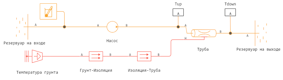
Description of the model
The pipe model for transporting heated oil includes
-
models of two tanks at the inlet and outlet (with atmospheric pressure and preset temperature and tank outlet cross-section),
-
constant flow pump,
-
two models for accounting for thermal conductivity (between oil and pipe material and between pipe and soil),
-
ground temperature model
-
and pipeline model (1000 m with standard parameters).
Let's run this model using command control:
engee.open(model_path)
data = engee.run("pipeline-geometry-for-heated-oil-transportation")
plot( data["Before the pipeline"].time, data["Before the pipeline"].value,
      label="Before the pipeline", lw=2 )
plot!( data["After the pipeline"].time, data["After the pipeline"].value,
      label="After the pipeline", lw=2 )
plot!( title="Dynamics of oil cooling at the pipeline outlet", titlefont=font(12),
       xlabel="Time, c", ylabel="Temperature, K", legend=:right)
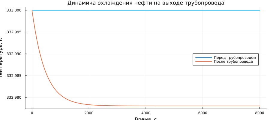
When passing 1000 m of a pipeline of a given geometry with specified heat loss parameters, the oil temperature dropped by only 0.02 degrees.
Conclusion
By running this model with different parameters, we can choose the optimal pipe diameter, at which the oil does not cool down too much in the specified area (1000 m). This is important to avoid solidification and ensure stable pumping without unnecessary heating costs. This approach allows you to design more economical and reliable pipelines, evaluating different options in advance without expensive experiments.
Bibliography
- Probert S. D., Chu C. Y. Optimal pipeline geometries and oil temperatures for least rates of energy expenditure during crude-oil transmission //Applied Energy. – 1983. – Vol. 14. – No. 1. – pp. 1-31.