Modeling of a conveyor belt
In this example, we will look at the calculation and modeling of a conveyor belt using physical modeling blocks.
Introduction
In general, the conveyor belt device can be represented as shown in the diagram.:
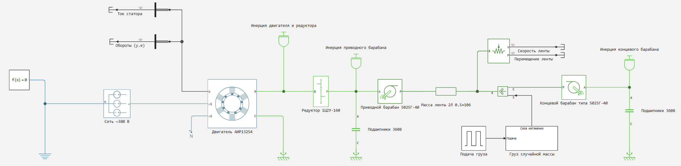
As an assumption for the final model, we will not take into account the dynamics of tension and sagging of the conveyor belt, therefore, the model can be simplified to several elements.:
-
electric drive,
-
gearbox,
-
drive drum with bearings,
-
end drum with bearings,
-
Conveyor belt.
-
cargo of variable mass.
Calculation of pipeline parameters
For an example of calculation and modeling, let's take the conveyor 5025-40, the equipment parameters of which will be selected according to [1].
Setting the length L of the pipeline:
L = 30; # Distance between reels [m]
Electric drive
The motor used in this example is asynchronous with a closed-loop rotor (AD KZR) AIR 132 S4. Power - 7.5 kW, rotation speed - 1455 rpm. It was calculated and modeled earlier, in the example of blood pressure parameterization.
Drums
The drums for the specified type of conveyor - drive and end have a standard size of 5025G-40. It defines the following characteristics necessary for physical modeling:
Dб = 250e-3; # Drum diameter [m]
Lб = 500e-3; # Drum length [m]
Mб = 58; # Drum weight [kg]
Jб = 0.5*Mб*(Dб/2)^2; # Moment of inertia of the drum [kg·m2]
In the model, the reels are represented by blocks:
-
inertia - to generate the torque of the drum,
-
wheel and axle - to convert rotational motion into translational motion (drive drum) and vice versa (end drum).
Reducer
One of the typical gearboxes for the 1TS2U-160 rear:
I = 31.5; # Gear ratio of the gearbox
J = 0.0227+0.01; # The moment of inertia of the gearbox and rotor AD, driven to the motor shaft [kg·m2]
ηр = 0.97; # Gearbox EFFICIENCY
In the model, it is described in two blocks:
-
gear transmission - it should be noted that this gearbox is two-stage, therefore, the direction of rotation of the input and output shafts coincide,
-
inertia - to generate the total torque of the motor rotor and gearbox shafts driven to the motor shaft.
Drum bearings
The type of bearings corresponding to a given drum is 3608. The following variables can be defined for them:
Tb = 12e-3; # The moment of friction of the bearing at rest [N·m]
Tc = 6e-3; # Sliding bearing friction moment [N·m]
Vc = Tc*0.05; # Coefficient of viscous friction [N·m/(rad/s)]
In the model, they are represented by blocks of rotational терния - with double coefficients and moments of friction (two bearings per drum axis).yu
Conveyor belt
Conveyor belt - general purpose, type 2L. Its parameters:
Bл = Lб; # Band width [m]
Lл = round((L*2+pi*Dб)*1.05); # Tape length [m]
mл = 3.75; # Specific gravity of the tape [kg/p.m.]
Mл = mл*Lл; # Belt weight [kg]
In the model, it is represented by the [mechanical mass] block (https://engee.com/helpcenter/stable/en/fmod-mechanical-translational-elements/mass.html ). The elasticity, tensile strength and damping effects of the tape are not taken into account.
Cargo
The load in the model is formed using the [force source] block (https://engee.com/helpcenter/stable/en/fmod-mechanical-translational-sources/force-source.html ) - with periodic delivery of random-value cargo.
Fгруза_max = 5e3; # Maximum tension of the belt from the load [N]
Fгруза_min = 1e3; # Minimum tension of the belt from the load [N]
The model takes into account the accumulation of cargo on the belt and the removal of cargo at the end of the conveyor after 51 seconds. The non-linearity of the characteristic of the movement of each load on the belt requires further more correct accounting.
The example model
The general view of the conveyor model is shown in the figure below.:
.png)
Let's run the model using software modeling control and pre-prepared functions for ease of working with the model and simulation results:
example_path = @__DIR__; # We get the absolute path to the directory containing the current script
cd(example_path); # Go to the example directory
include("useful_functions.jl"); # We connect the Julia script with auxiliary functions
simout = get_sim_results("conveyor.engee", example_path) # running the simulation
Simulation results
Engine
We obtain the variables of the signals recorded in the model, measured on the engine:
t = thin(get_sim_data(simout, "Stator current", 1, "time"), 50);
Is = thin(get_sim_data(simout, "Stator current", 1, "value"), 50);
n = thin(get_sim_data(simout, "Revolutions (units)", 1, "value"), 50);
Let's plot these variables:
gr(fmt=:png, aspectratio=:auto, xlims=:auto, ylims=:auto, size = (900,400))
I_graph = plot(t, Is; label = "I(t)", title = "Stator current", ylabel = "I [A]", xlabel = "t [s]")
n_graph = plot(t, n; label = "n(t)", title = "Rotor speed", ylabel = "n [units]", xlabel = "t [s]")
plot(I_graph, n_graph)
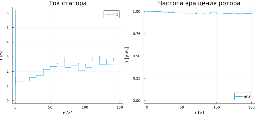
The graphs show how the stator current periodically increases by a variable amount, while the rotor frequency decreases - this indicates an increase in the load on the motor shaft. After 51 seconds, you can see that the load stops increasing - loads continue to arrive on the belt, but those who hit it first are already being removed from the conveyor.
Conveyor belt
We will get variables from the signals recorded in the model on the conveyor belt:
Vл = thin(get_sim_data(simout, "Tape speed", 1, "value"), 50);
Sл = thin(get_sim_data(simout, "Moving the tape", 1, "value"), 50);
Let's plot these variables:
gr(fmt=:png, aspectratio=:auto, xlims=:auto, ylims=:auto, size = (900,400))
V_graph = plot(t, Vл; label = "V(t)", title = "Tape speed", ylabel = "V [m/s]", xlabel = "t [s]")
S_graph = plot(t, Sл; label = "S(t)", title = "Moving the tape", ylabel = "S [m]", xlabel = "t [s]")
plot(V_graph, S_graph)
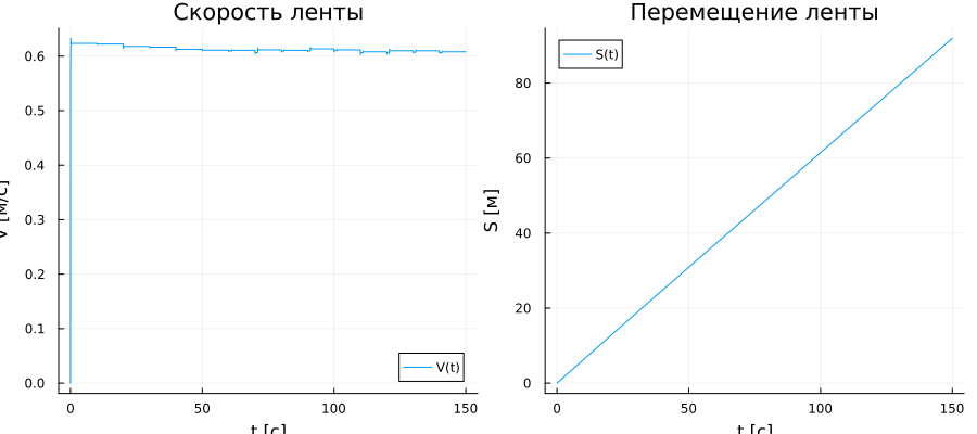
The speed of the belt is directly proportional to the rotational speed of the motor shaft, the average value corresponds to the speed determined by the reference book for this type of conveyor:
import Pkg; Pkg.add("Statistics")
using Statistics
Vp_sr = round(mean(Vp)*100, digits=2)
println("The average speed of the conveyor belt is $Vl_sr cm/s")
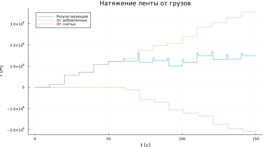
Loads on the conveyor
At the end of the analysis of the simulation results, we will analyze the tension forces of the belt from the loads on the belt.:
Tmain = thin(get_sim_data(simout, "Load tension force", 1, "value"), 50);
Tsub = thin(get_sim_data(simout, "Removed loads.1", 1, "value"), 50);
Tadd = thin(get_sim_data(simout, "Added loads.main_out", 1, "value"), 50);
Let's plot the recorded signals:
gr(aspectratio=:auto, xlims=:auto, ylims=:auto, size = (900,500))
plot(t, Tmain; label = "The resulting", title = "Belt tension from loads", ylabel = "T [H]", xlabel = "t [s]")
plot!(t, Tadd; label = "From added", ls=:dot)
plot!(t, -Tsub; label = "From the removed", ls=:dot)
Conclusion
As a result of the calculation and modeling, a physical model of a conveyor belt with cargo delivery was developed that takes into account the dynamics of belt tension from cargo. In further work on the project, you can proceed to the development of a conveyor management system.
Literature
- Stationary general-purpose conveyor belts with a rubber-cloth belt. Catalog. Part I. Equipment // JSC "Belokholunitskiy zavod" - 2002