Simulation of ball bounce in 1D solver
Let's build a 1D model of the dynamics of a simple mechanical system: a model of the interaction of a material point with the earth's surface when falling under the influence of gravity.
Description and launch of the model
Let's imagine the simplest scenario for calculating the dynamics of an object interacting with a surface.
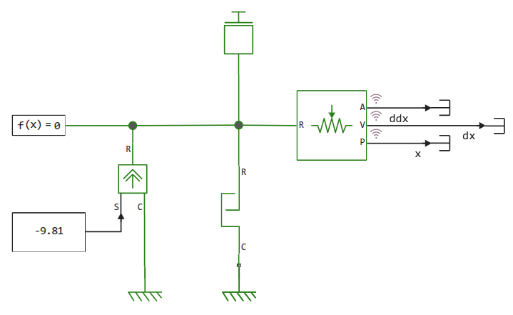
An object is a material point that is affected by gravity, and when it collides with a surface, it has an acceleration pulse.
The Translational Hard Stop block is responsible for interaction with the surface. One of the useful effects of using 1D modeling is that, without additional effort, we get a slightly more complex model of the support reaction than a perfectly elastic rebound.
Let's run the model and study the results.:
model = engee.open("physical_bouncing_ball.engee")
data = engee.run(model)
plot(
    plot( data["x"].time, data["x"].value, c=1, label="Position" ),
    plot( data["dx"].time, data["dx"].value, c=2, label="Speed" ),
    plot( data["ddx"].time, data["ddx"].value, c=3, label="Boost" ),
    layout=(3,1), lw=3
)
The model is assembled as simply as possible, nothing has been changed in the parameters of the physical or global solver, except for switching it to the "integration by variable steps" mode so that all acceleration pulses are visible on the graph.
Conclusion
This approach is an ideal start for modeling vertical motion. When you need to quickly test a concept or understand the basic dynamics of a system, these three blocks provide a ready-made solution without unnecessary complexity.