Simulation of hydraulic shock
In this example, we will explore how to model гидроудар in a long pipe using Isothermal liquid (IL) library blocks.
The flow of liquid in the pipe is controlled by a valve. First, the control system smoothly opens the valve, increasing the flow rate, but maintaining the stationary nature of the flow. Then, when the valve is abruptly closed (0.1 s), we can observe the effect of a water hammer.
Description of the model
At the top level, the model looks like this:
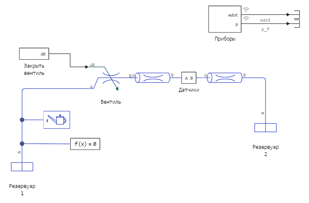
The pipeline connects two reservoirs, in the first one a pressure of 6 atmospheres is maintained. The liquid will flow into the second tank, the pressure in which is also constant and equal to 5 atmospheres.
Between two pipes with a length of 25 meters there is a subsystem "Sensors", where flow and pressure sensors are located. To preserve the topology of the model, the plotting module is placed in a separate subsystem "Devices". Data can be filtered there, but in this model we only multiply the total pressure in pascals by a constant to get readings in atmospheres.
The operation of the valve control unit depends on the state variable sqitching_mode, which can take the value "Fast" or "Slow". The rapid shut-off of the flow puts the system into a very active non-stationary mode, which we will demonstrate.
switching_mode = "Fast";
To simulate the valve, we use the block Variable Local Restriction (IL), pipes are represented by blocks Pipe (IL). To see the effect of a water hammer, it is necessary that the pipe model allows you to simulate the compressibility and inertia of a liquid (by default, pipes do not take inertia into account, it must be enabled in the block settings Pipe (IL)).
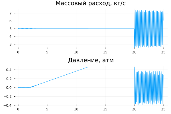
Simulation of rapid valve shut-off
In this variant of the model, the step function that sets the valve overlap is smoothed using the transfer function. . As a result, we are witnessing a rather abrupt transition process.
# Set the model to the fast switching mode
switching_mode = "Fast";

# Download and run the model
modelName = "water_hammer"
model = modelName in [m.name for m in engee.get_all_models()] ? engee.open( modelName ) : engee.load( "$(@__DIR__)/$(modelName).engee");
data = engee.run( modelName )
And, as we can see in the graphs, after a long period of steady operation, the pipes begin to experience sudden pressure surges, and the displaced mass of liquid fluctuates just as sharply between 3 and 5 kg/s.
gr()
plot(
    plot( data["p_f"].time, data["p_f"].value, leg=false, title="Mass flow rate, kg/s" ),
    plot( data["mdot"].time, data["mdot"].value, leg=false, title="Pressure, atm" ),
    layout=(2,1)
)
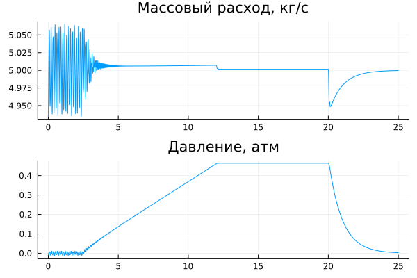
Simulation of slow valve shut-off
If you control the valve slowly enough (smoothing the step using the transfer function ), then we observe a smooth transition process.
# Let's set the model to the fast switching mode
switching_mode = "Slow";

# Let's run another version of the model
data = engee.run( modelName )
gr()
plot(
    plot( data["p_f"].time, data["p_f"].value, leg=false, title="Mass flow rate, kg/s" ),
    plot( data["mdot"].time, data["mdot"].value, leg=false, title="Pressure, atm" ),
    layout=(2,1)
)
Conclusion
We have obtained a fairly convincing demonstration of the effect of hydraulic shock, using a minimum of auxiliary blocks. We built a system with two operation options (fast and slow valve closure) and brought out the dashboard through a separate subsystem, successfully using the blocks From and Goto.
To make the model more visual, it would be possible to add more pipeline segments and measure the pressure between them, or simulate a damped reservoir.