DC motor with electrical and mechanical parameters

This example will demonstrate a model of a DC motor with electrical and mechanical parameters. The process of launching the model from the script development environment using command control, as well as visualization of the simulation results, will be shown. In the simulation, an alternating torque acts on the shaft of the electric motor.

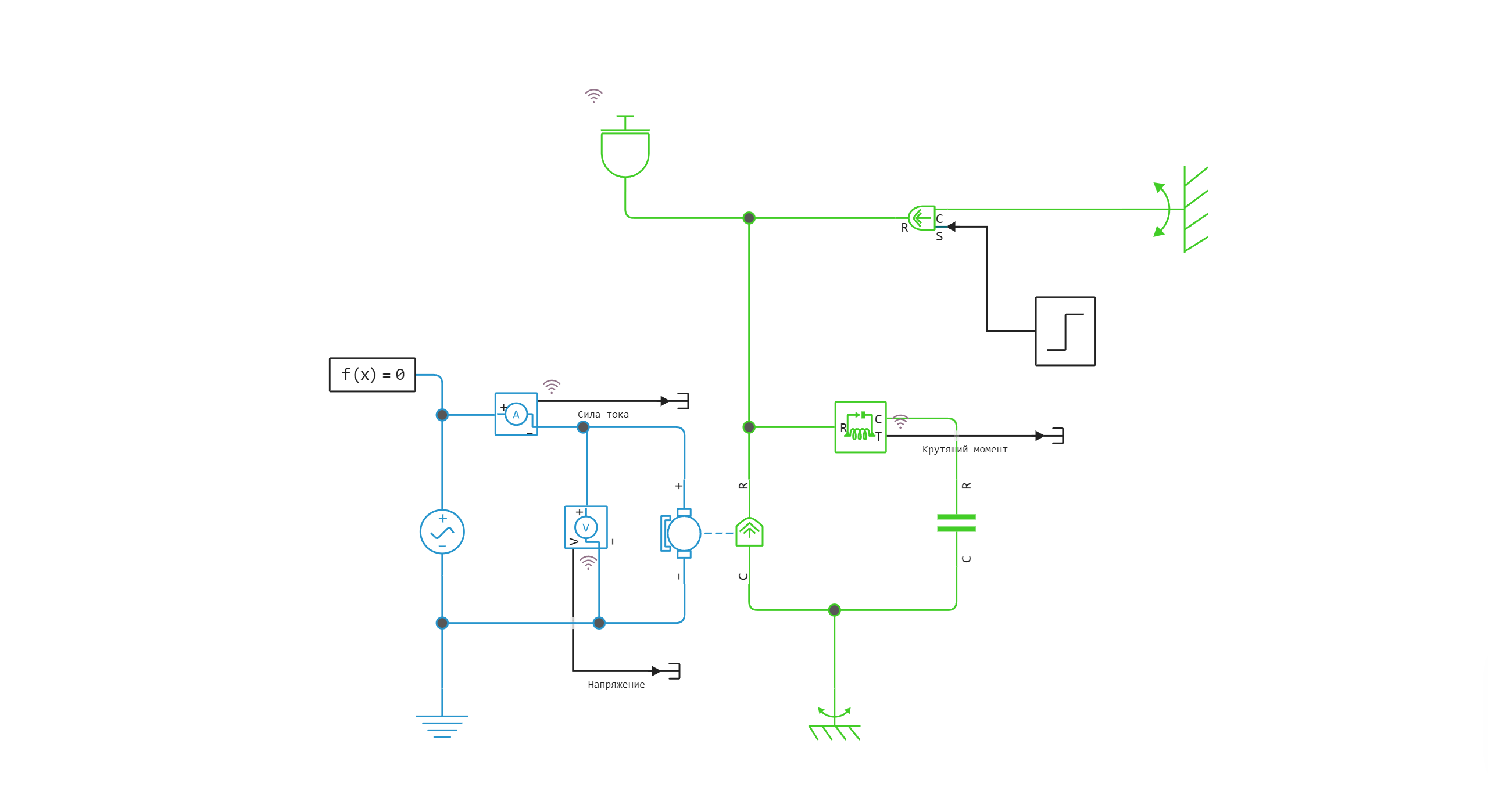
General view of the models

The Engee model:

Defining a function to load and run the model:

function start_model_engee()
    try
        engee.close("dc_motor_default", force=true) # закрытие модели 
        catch err # в случае, если нет модели, которую нужно закрыть и engee.close() не выполняется, то будет выполнена её загрузка после catch
            m = engee.load("/user/start/examples/physmod/dc_motor_default/dc_motor_default.engee") # загрузка модели
        end;

    try
        engee.run(m, verbose=true) # запуск модели
        catch err # в случае, если модель не загружена и engee.run() не выполняется, то будут выполнены две нижние строки после catch
            m = engee.load("/user/start/examples/physmod/dc_motor_default/dc_motor_default.engee") # загрузка модели
            engee.run(m, verbose=true) # запуск модели
        end
end

start_model_engee (generic function with 1 method)

Loading, running the model, and recording the results

try
    start_model_engee() # загрузка и запуск модели
    catch err
    end;
sleep(5)
#data1 = collect(simout) # выделение из переменной simout данных, описывающих ток коллектора и напряжение коллектор-эмиттер
#Vce = collect(data1[2]) # запись данных о напряжении коллектор-эмиттер в переменную
#Ic1 = collect(data1[3]); # запись данных о токе коллектора в переменную

Building...
Progress 100%

Writing signals to the data variable:

data = collect(simout)

7-element Vector{WorkspaceArray}:
 WorkspaceArray("dc_motor_default/Inertia.flange.T")
 WorkspaceArray("dc_motor_default/Крутящий момент")
 WorkspaceArray("dc_motor_default/Inertia.T")
 WorkspaceArray("dc_motor_default/Сила тока")
 WorkspaceArray("dc_motor_default/Напряжение")
 WorkspaceArray("dc_motor_default/Inertia.flange.w")
 WorkspaceArray("dc_motor_default/Inertia.w")

Recording data on the current and torque on the motor shaft in the variables current and torque:

torque = collect(data[2])
current = collect(data[4]);

Visualization of results

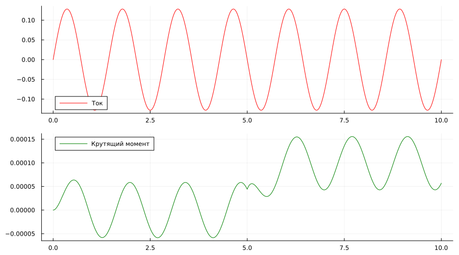
Output of graphs of the dependence of current and torque on time:

p1 = plot(current[:,1], current[:,2], label="Ток", color="red")
p2 = plot(torque[:,1], torque[:,2], label="Крутящий момент", color="green")
plot(p1, p2, layout=(2,1))

Conclusions:

In this example, tools for command management of the model were used. The simulation results using simout were recorded in the corresponding variables, as well as visualized using interactive graphs from the Plots library.