Investigation of the properties of a compressible gas
In this example, we will use the piston model and plot the graphs of the gas compression experiment.
Description of the model
The main element of the model is the piston block Translational Mechanical Converter. A negative displacement of the piston rod means that it is compressed and leads to an increase in temperature and pressure in the outlet channel.
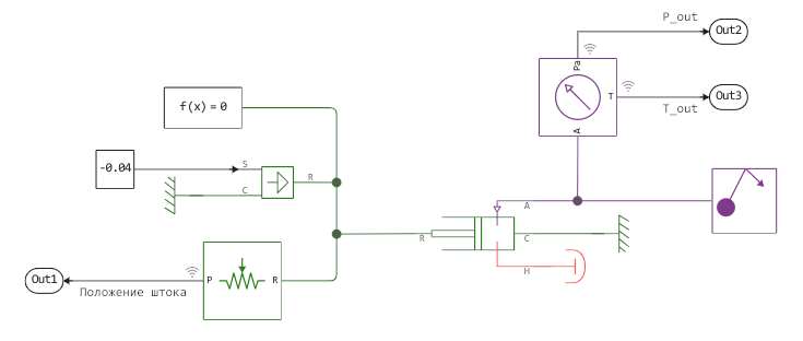
Additional units are responsible for controlling the condition of the piston and measuring this condition.:
- the movement of the rod is carried out by the action of
Translational Velocity Source - Motion sensor
Absolute Translational Motion Sensormeasures the position of the stem - Pressure and temperature sensor
Absolute Pressure & Temperature Sensor (G)allows you to measure the properties of the gas at the piston outlet - block
Gas Properties (G)sets the properties of the working fluid of our model.
The model can work with an ideal gas, with semi-ideal and real gas models.
The piston has a limit position (equal to 0.0) and an initial position (Initial interface displacement), set to 0.5 m.
When the zero position is reached, the pressure inside the piston will be equal to the value set in its properties. Dead volume (in the model, it is equal to 1e-5 m^3), the rod cannot move further.
Rod control
In this model, the movement of the rod is set by a constant speed unit. With this control, the movement of the rod will be uniform, translational and will not take into account the oncoming impact from the compressed gas. In reality, an approximate situation may arise when the reaction of the gas to compression is negligible compared to the force exerted on the piston rod, and the piston itself is structurally indestructible.
In this case, connecting the force source to the piston rod results in an unsolvable system of equations.
If the initial position of the rod is zero, negative movement of the piston is not possible. When solving such a system, the integrator will reduce the step until an error occurs. DtLessThanMin.
Transmitting a "positive value" of the speed to the block Translational Velocity Source it leads to a stretching of the rod and a decrease in pressure and temperature at its outlet. Change the block value Constant on the positive side to make sure of it.
Launching the model
# We will load the model if it is not already open on the canvas.
if "gas_actuator_model" ∉ getfield.(engee.get_all_models(), :name)
    engee.load( "$(@__DIR__)/gas_actuator_model.engee");
end

model_data = engee.run( "gas_actuator_model" );
Let's plot the state of the gas.
gr()
pos = collect( model_data["Stem position"] )
P_out = collect( model_data["P_out"] )
T_out = collect( model_data["T_out"] )
plot(
    layout=(2,1),
    plot( pos.time, pos.value, title="Rod movement", leg=false, c=1),
    plot( plot( P_out.time, P_out.value, title="Pressure", leg=false, c=2 ),
          plot( T_out.time, T_out.value, title="Temperature", leg=false, c=3 ) )
)
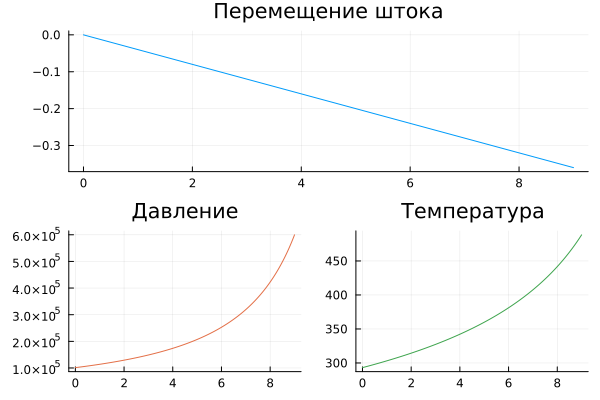
The upper graph shows the movement of the rod from its initial position (and not the position relative to the zero point).
If the simulation time is increased beyond 10 seconds, the rod position will reach zero and the simulation will stop with an error. To avoid this, there are more complex models based on Translational Mechanical Converter For example , the block Single-Acting Actuator (G).
Conclusion
This small model allows us to understand the work of one of the basic "building blocks" in gas dynamic models. This block underlies many other more complex node models, such as linear gas drives and compressors.