Simulation of an inductor with hysteresis.
This example shows how changing the coefficients of the Giles-Atherton magnetic hysteresis equation affects the resulting B-H curve. The simulation parameters are configured to perform four complete alternating current cycles with the initial field strength (H) and magnetic flux density (B) set to zero.
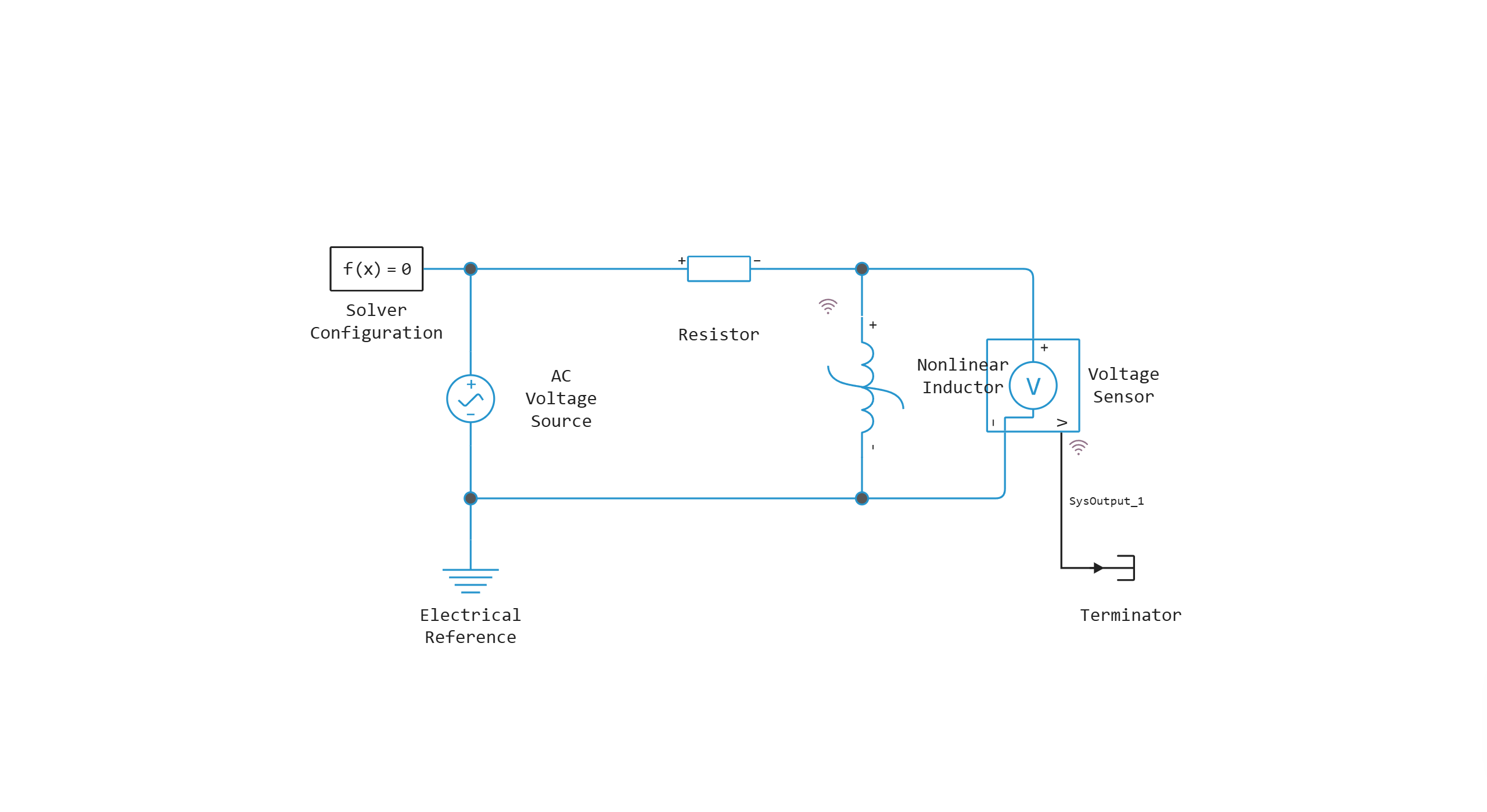
Model diagram:
Defining the function to load and run the model:
function start_model_engee()
    try
        engee.close("inductor_with_hysteresis", force=true) # closing the model
        catch err # if there is no model to close and engee.close() is not executed, it will be loaded after catch.
            m = engee.load("$(@__DIR__)/inductor_with_hysteresis.engee") # loading the model
        end;

    try
        engee.run(m) # launching the model
        catch err # if the model is not loaded and engee.run() is not executed, the bottom two lines after catch will be executed.
            m = engee.load("$(@__DIR__)/inductor_with_hysteresis.engee") # loading the model
            engee.run(m) # launching the model
        end
end
Launching the model:
try
    start_model_engee() # running the simulation using the special function implemented above
    catch err
    end;
Output of simulation results from the simout variable:
res = collect(simout)
Writing results to variables:
H = collect(res[4]) # field strength
B = collect(res[5]) # magnetic flux density
using Plots
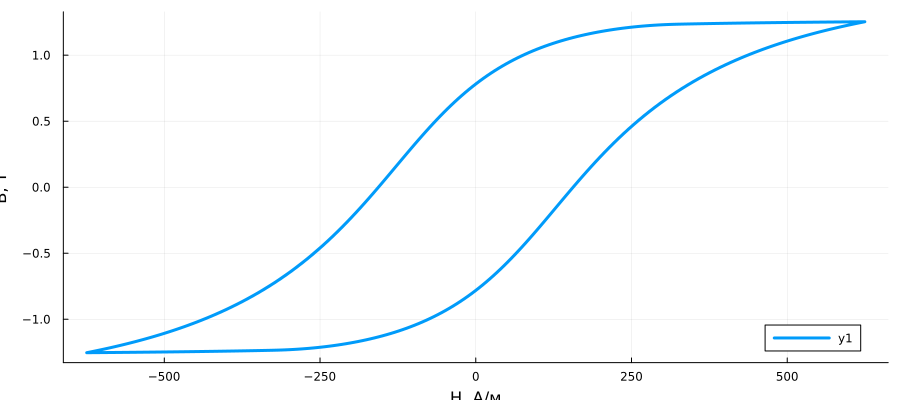
plot(H[100:end,2], B[100:end,2], linewidth=3, xlabel= "H, Vehicle", ylabel= "B, T", legend=:bottomright)
Determination of a new reverse magnetization coefficient:
Output of the Nonlinear Inductor block parameters:
engee.get_param("inductor_with_hysteresis/Nonlinear Inductor")
We redefine the values of the coefficients of the magnetic hysteresis equation using the function set_param! Hidden under a mask:
engee.load("$(@__DIR__)/inductor_with_hysteresis.engee")
# @markdown Reversible magnetization coefficient:
c = 0.2 # @param {type:"slider", min:0, max:1, step:0.1}
# @markdown Volume ratio:
K = 200.0 # @param {type:"slider", min:0, max:1000, step:1}
# @markdown Cross-domain coupling coefficient:
alpha = 0.0001 # @param {type:"slider", min:0, max:0.001, step:0.0001}
engee.set_param!("inductor_with_hysteresis/Nonlinear Inductor", "c" => c)
engee.set_param!("inductor_with_hysteresis/Nonlinear Inductor", "K" => K)
engee.set_param!("inductor_with_hysteresis/Nonlinear Inductor", "alpha" => alpha)
engee.run("inductor_with_hysteresis")
res1 = collect(simout)
H1 = collect(res1[7])
B1 = collect(res1[9])
engee.close("inductor_with_hysteresis", force = true)
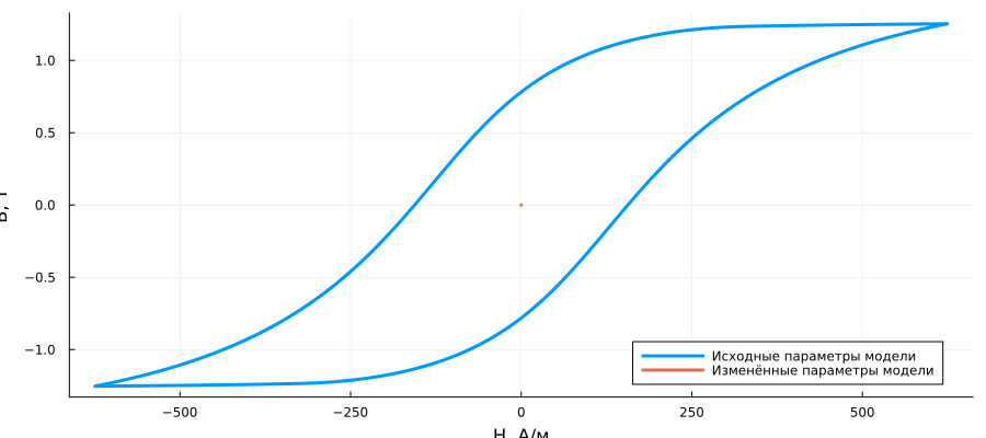
plot(H[100:end,2], B[100:end,2], label = "Initial parameters of the model", xlabel= "H, Vehicle", ylabel= "B, T", linewidth=3)
plot!(H1[100:end,2], B1[100:end,2], label = "Changed model parameters", legend=:bottomright, linewidth=3)
Conclusions:
In this example, a simulation of an inductor model with hysteresis was performed using software control. The graphs show how the individual coefficients of the Giles-Atherton equations affect the hysteresis curve.