Simulation of an LC oscillator based on the Kolpits scheme
This example shows the implementation of a Colpits oscillator circuit with a nominal frequency of 9 MHz. The oscillation frequency is given by the formula:
LC oscillators have good frequency selectivity due to higher quality levels compared to RC oscillators.
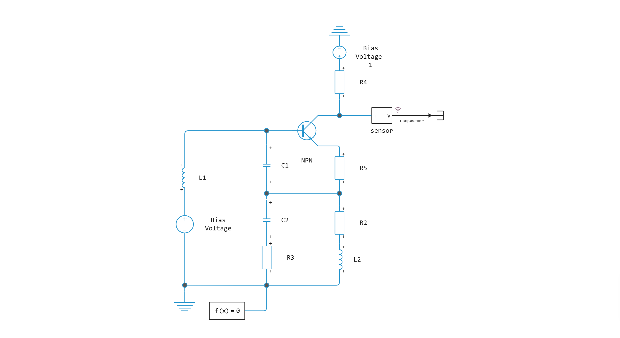
Model diagram:
Defining a function to load and run the model:
In [ ]:
function start_model_engee()
    try
        engee.close("lc_oscillator", force=true) # closing the model
        catch err # if there is no model to close and engee.close() is not executed, it will be loaded after catch.
            m = engee.load("$(@__DIR__)/lc_oscillator.engee") # loading the model
        end;

    try
        engee.run(m) # launching the model
        catch err # if the model is not loaded and engee.run() is not executed, the bottom two lines after catch will be executed.
            m = engee.load("$(@__DIR__)/lc_oscillator.engee") # loading the model
            engee.run(m) # launching the model
        end
end
Out[0]:
Running the simulation
In [ ]:
try
    start_model_engee() # running the simulation using the special function implemented above
    catch err
    end;
Writing from simout to voltage signal variables:
In [ ]:
res = collect(simout)
V = collect(res[1])
Out[0]:
Visualization of simulation results
In [ ]:
using Plots
In [ ]:
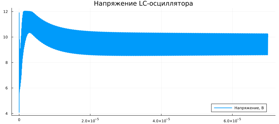
plot(V[:,1], V[:,2], label="Voltage, V", linewidth=2, title="LC Oscillator voltage")
Out[0]:
In [ ]:
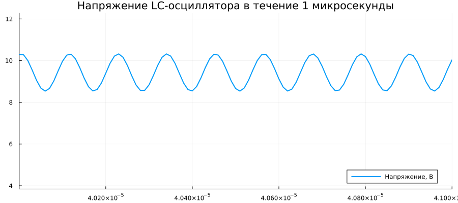
plot(V[:,1], V[:,2], label="Voltage, V", linewidth=2, xlim=(4e-5, 4.1e-5), title="LC oscillator voltage for 1 microsecond")
Out[0]: