Model mass-spring-damper
In this example, we will study two approaches to modeling a classical dynamic model that includes a single point object with a given mass connected to a support using a spring and a damper. Let's run the models and compare the results when choosing solvers with constant and variable integration steps.
Pkg.add(["Interpolations"])
gr()
Description of models
A dynamic system, including a mass, a spring, and a damper, is very often used to study the nature of oscillatory processes, kinematics, and effects of chaotic motion (if there are several objects), or numerical integration methods.
We will consider the directional model. msd_causal.engee, which performs numerical integration of the equation .
.png)
You can clearly see that if you express the equation for acceleration of the load from this formula, then it is exactly what comes to the input of the integrator. .
The second model msd_acausal.engee It was created from non-directional (acausal) blocks of the Engee physical modeling library. In the upper part there is a sensor that measures the movement of the mass relative to the fulcrum, as well as a block SolverConfiguration which indicates to the global solver of the model that the signals and blocks connected to it will have its own integrator with its own settings.
.png)
At the bottom of the model there is a group of elements resembling standard educational illustrations. it is connected to the support by means of a spring with rigidity and dampers with an absorption coefficient (the changeable parameters are specified in the properties of these blocks).
Due to the graphical nature of the model, these elements are easy to arrange in a variety of ways, connect in parallel or in series, or duplicate multiple times.
Setting model parameters
Both models use identical variable parameters: cargo weight m, spring stiffness k and the absorption coefficient of the damper b.
b,k,m = 1,2,3;
When the necessary variables are created, you can manage the models by changing the values of the variables in the Variables Window. With values of b=1, k=2, m=3 we should observe a rather slow, inertial process with noticeable attenuation.
Downloading and exploring models
Using a one-line command, we will either load (load), or open the already loaded model (open). Here we use the syntax of one-line conditional operators x = условие ? если_истинно : если_ложно.
# One-line command to open/load a model
mc = "msd_causal" in [m.name for m in engee.get_all_models()] ? engee.open( "msd_causal" ) : engee.load( "$(@__DIR__)/msd_causal.engee" );
ma = "msd_acausal" in [m.name for m in engee.get_all_models()] ? engee.open( "msd_acausal" ) : engee.load( "$(@__DIR__)/msd_acausal.engee" );
Let's see what integrator parameters are prescribed in both models.
using DelimitedFiles, DataFrames

# Let's collect the parameters of the models
mc_dict = engee.get_param( "msd_causal" );
ma_dict = engee.get_param( "msd_acausal" );
df_causal = DataFrame("Property"=>collect(keys(mc_dict)), "The directional model"=>collect(values(mc_dict)))
df_acausal = DataFrame("Property"=>collect(keys(ma_dict)), "The physical model"=>collect(values(ma_dict)))

# A table for comparing model parameters
df = outerjoin(df_causal, df_acausal, on="Property")

# Let's filter out the properties of the model that we are interested in
params_to_display = ["StartTime", "StopTime", "SolverType", "SolverName", "FixedStep"]
df[in(params_to_display).(df."Property"), :]
We can see that both models have the same integrator settings.
In fact, the algorithm for the numerical solution of the physical model is specified in the block Solver Configuration, but the upper-level integrator of the model, which receives signals from the physical subsystem and returns measurements in the form of vectors, performs their sampling with a constant step 0.01 with.
Execution of models with variable pitch
Let's run the models and save the results to variables. rc and ra for directional and physical models, respectively.
rc = engee.run( "msd_causal" );
ra = engee.run( "msd_acausal" );
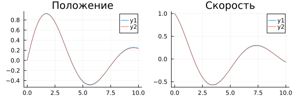
Comparison of execution results:
plot( rc["p"].time, rc["p"].value, title="Position" )
p_pos = plot!( ra["p"].time, ra["p"].value )

plot( rc["v"].time, rc["v"].value, title="Speed" )
p_vel = plot!( ra["v"].time, ra["v"].value )

plot( p_pos, p_vel, size=(600,200) )
Since the data was collected with the same discretization in both models, we can look at the difference between the results of the algorithmic and physical models.
using LaTeXStrings
d_pos = plot( ra["p"].value - rc["p"].value, title=L"\varepsilon_{position}", legend=false)
d_vel = plot( ra["v"].value - rc["v"].value, title=L"\varepsilon_{speed}", legend=false )

plot( d_pos, d_vel, size=(600,200) )
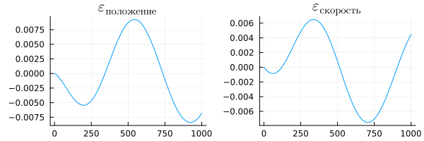
The difference between the results is obviously very small, the order of the value is .
Let's see what happens if we switch the "algorithmic" model to the same mode in which the solver of the physical model works.
Let's switch to a constant-step solver.
Switch the mode of operation of both models. Now all solvers select the optimal step size and output data at different sampling rates.
# Let's set up the directional model so that it is solved with a variable integration step.
engee.set_param!( "msd_causal", "SolverType"=>"variable-step" )
engee.set_param!( "msd_acausal", "SolverType"=>"variable-step" )

# Let's launch the models
rc = engee.run( "msd_causal" );
ra = engee.run( "msd_acausal" );
To compare graphs with different resolutions, we will need interpolation.
using Interpolations
# Creating two objects to interpolate the position and velocity of the causal model
rc_p_interp_linear = linear_interpolation(rc["p"].time, rc["p"].value)
rc_v_interp_linear = linear_interpolation(rc["v"].time, rc["v"].value)

# Calculating the difference between interpolation and calculation of the physical system
e_pos = plot( ra["p"].time, ra["p"].value - rc_p_interp_linear.(ra["p"].time), title=L"\varepsilon_{position}", legend=false )
e_vel = plot( ra["v"].time, ra["v"].value - rc_v_interp_linear.(ra["v"].time), title=L"\varepsilon_{speed}", legend=false )

plot( e_pos, e_vel, size=(600,200) )
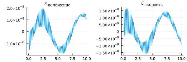
This time, the difference between the physical model and the directional model is much smaller - the discrepancy has an order of magnitude. .
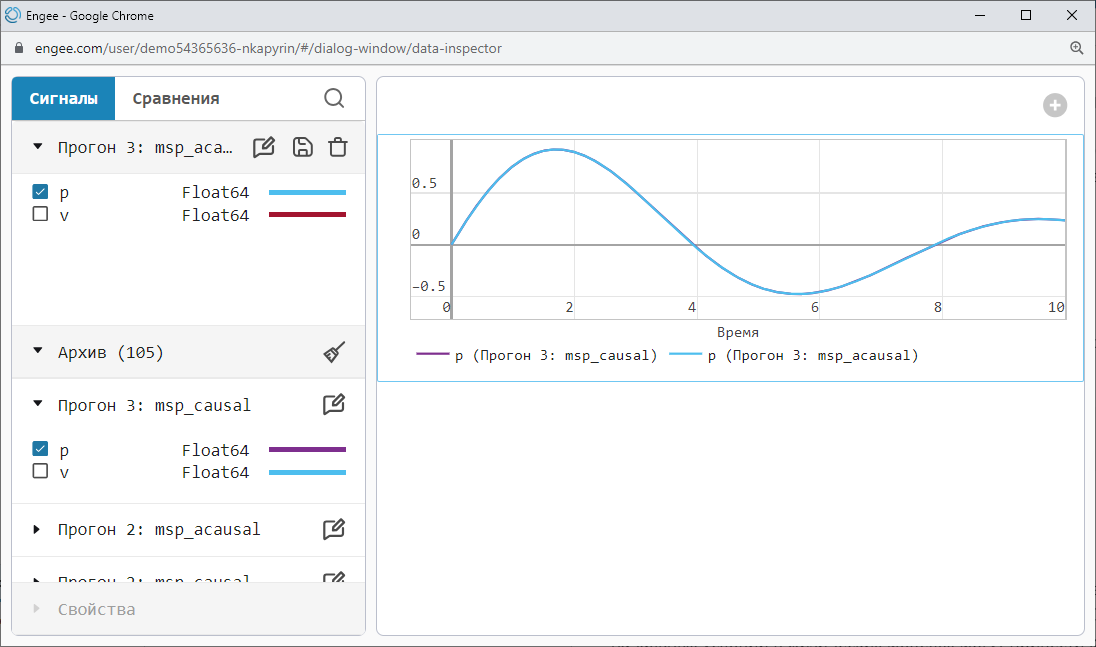
Engee has a built-in Data Inspector that allows you to compare different launch results with each other.
.png)
Closing models without saving
If we later want to run this example again from the very beginning, then we need to close the models without saving the changes made.
engee.close( "msd_causal", force=true );
engee.close( "msd_acausal", force=true );
Conclusion
Unlike directional models, physical models, as a rule, cannot be solved using solvers with a constant integration step. Difficulties in substituting implicit initial conditions can lead to numerical instability, such as infinite gradients.
The ability to explore models of different nature and apply various integration methods in an automated manner allows us to choose the optimal solution in both respects: the most understandable modeling formalism and the most stable solver.