Modeling data processing

In this example, let's look at how to get simulation data from a model, as well as how to process the received data correctly and efficiently in Engee scripts.

Introduction

There are two ways to ensure that the recorded model signals immediately enter the workspace during the simulation process.:

Use the [simout] variable(https://engee.com/helpcenter/stable/en/feature/about-simout.html )
Use the [To Workspace] blocks(https://engee.com/helpcenter/stable/en/base-lib-sinks/to-workspace.html )

Each has its own pros and cons, and specific approaches to use.

1. We use `simout`

1.1. Getting a variable

So that the necessary data from the model is written to a variable simout, you need to do the following:

Set the necessary signals for recording.
Enable the option "Save simulation results to your desktop область".

Recommendation

For convenience of operation, it is recommended to define a name for the recorded signals.

Opportunity

When setting signals for recording and de-recording, the recommended tool is model data editor.

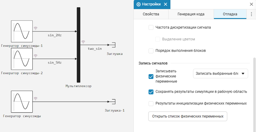
Now, after executing the model, we get a variable in the workspace simout:

model1_path = "$(@__DIR__)/simulation1.engee" 
engee.load(model1_path) |> engee.run; # uploaded and executed the model
engee.close(engee.gcm(), force=true) # the model was closed

simout

SimulationResult(
    run_id => 8,
    "simulation1/sin_5Hz" => WorkspaceArray{Float64}("simulation1/sin_5Hz")
,
    "simulation1/sin_2Hz" => WorkspaceArray{Float64}("simulation1/sin_2Hz")
,
    "simulation1/Sinusoid generator.1" => WorkspaceArray{Float64}("simulation1/Sinusoid generator.1")
,
    "simulation1/two_sin" => WorkspaceArray{Vector{Float64}}("simulation1/two_sin")

)

1.2. Variable processing `simout`

In the received variable simout, in the dictionary dictthe pairs key (signal name) => value (signal - time and values/vector of values) are stored:

# we get all the names of the signals from simout
dict_keys = simout.dict |> keys |> collect

4-element Vector{String}:
 "simulation1/sin_5Hz"
 "simulation1/sin_2Hz"
 "simulation1/Sinusoid generator.1"
 "simulation1/two_sin"

Values for the first key - simulation/sin_5Hz they will look like this:

collect(simout.dict["simulation1/sin_5Hz"])

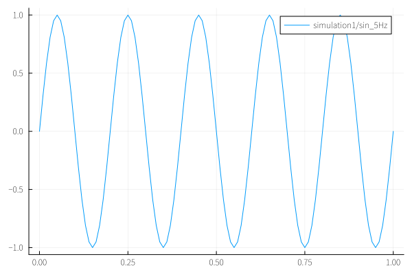
That is, in the meaning of the dictionary dict for the name of our signal simulation/sin_5Hz the object is stored WorkspaceArray with fields time and value. By accessing these fields, you can get the timestamps of the signal and the values themselves and plot a graph.:

t1 = simout.dict["simulation1/sin_5Hz"].time
val1 = simout.dict["simulation1/sin_5Hz"].value
gr(format=:png)
plot(t1, val1; label="simulation1/sin_5Hz")

1.3. Vector signal in `value`

The signal that we took to construct above was scalar - at one point in time, one value of the type was recorded Float64.
Consider another case where the signal simulation/two_sin - vector of values Float64:

simout.dict["simulation1/two_sin"].value[1] # we get the first element from the array of values of the simulation/two_sin signal

2-element Vector{Float64}:
 0.0
 0.0

As you can see, this is a vector of two values. The field will tell us the same thing. dimension the dictionary dict

simout.dict["simulation1/two_sin"].dimension # getting the value stored in the dimension field

(2,)

It follows from this: the dimension of the field values value - 2×1. And you won't be able to build them in the same way as before.:

t2 = simout.dict["simulation1/two_sin"].time
val2 = simout.dict["simulation1/two_sin"].value

plot(t2, val2; label="simulation1/two_sin")

print device already activated
print device already activated

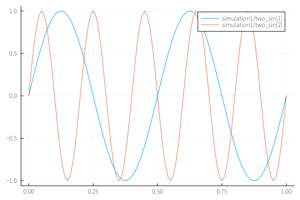
To get indexed arrays of individual signals and build them, we use getindex():

val2_1 = getindex.(val2, 1)
val2_2 = getindex.(val2, 2)

plot(t2, val2_1; label="simulation1/two_sin[1]")
plot!(t2, val2_2; label="simulation1/two_sin[2]")

print device already activated

1.4. Unnamed signal

If the name of the signal on the signal line was not determined during the simulation, the name of the signal in simout it will be determined by the name of the block and the port number from which it originates.

collect(simout.dict["simulation1/Sinusoid generator.1"])

Recommendation

This option is certainly working, but compared to named signals, it is less beautiful, more difficult to identify, and less convenient to process.

1.5. Thinning

The dimension of the arrays that we pass to plot() to build a graph, it is only:

simout.dict["simulation1/sin_5Hz"].value |> size # we determine the dimension of the vector of values of the simulation1/sin_5Hz signal

(101,)

101 elements in a vector that is in gr() the backend Plots, and even with the image format format = :png it is displayed on the graph fairly quickly.

Warning

For example, if you try to build an image svg in the interactive backend plotlyjs() for a vector of 100,000 elements, you will have to use significantly more resources and time.

If not every point is important for visualization, you can use the simplest option - lazy slices WorkspaceArray:

simout.dict["simulation1/sin_5Hz"].value[1:2:end]  |> size # we obtain a vector of signal values in increments of 2 and define a new dimension

(51,)

Lazy array slices allow you to use not all values for construction, but in steps of 2 ([1:2:end]) or otherwise ([1:3:end], [1:4:end], [1:5:end] and so on).

A lazy slice will also help to highlight the beginning of the signal ([1:20]) or the end ([40:end]).

Warning

This approach is convenient for thinning out constant, slightly changing, and harmonic signals. When thinning the latter, it is necessary to use Kotelnikov's theorem - the maximum frequency in the signal after thinning must be less than half of the new sampling frequency in order to fulfill the Nyquist condition.

Recommendation

For signals with non-periodic transients, more flexible decimation methods should be used, estimating signal changes and decimating based on the dynamics of its change.

2. We use the To Workspace blocks

2.1. Getting variables

In order for the necessary data from the model to be recorded in the workspace, you need to do the following:

Set the [ToWorkspace] block for each recorded signal (array)(https://engee.com/helpcenter/stable/en/base-lib-sinks/to-workspace.html ) (To the workspace).
Give names of variables written in blocks

Critical

In the second step, you need to be extremely careful - the variable name in the block must be set taking into account [the rules for naming variables] (https://engee.com/helpcenter/stable/en/julia/manual/variables.html ) Julia.

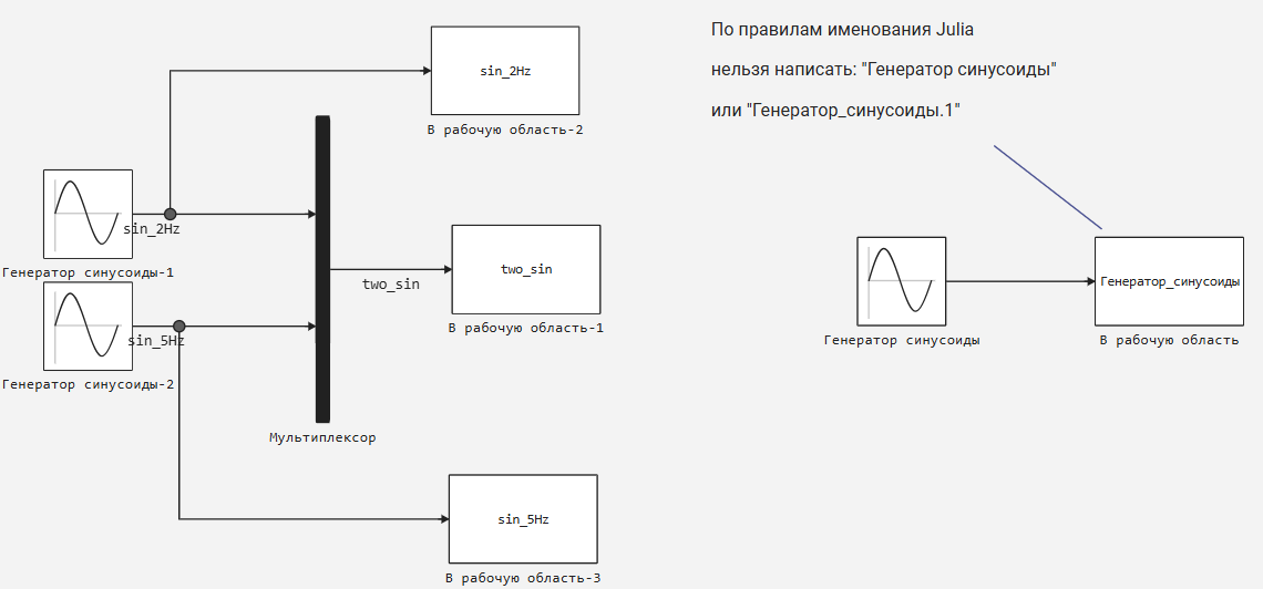
Now, after executing the model, we get variables in the workspace with the names specified in the blocks.

model2_path = "$(@__DIR__)/simulation2.engee" 
engee.load(model2_path) |> engee.run; # uploaded and executed the model
engee.close(engee.gcm(), force=true) # the model was closed

sin_2Hz, sin_5Hz, two_sin, Sinusoid oscillator

(WorkspaceArray{Float64}("sin_2Hz"), WorkspaceArray{Float64}("sin_5Hz"), WorkspaceArray{Vector{Float64}}("two_sin"), WorkspaceArray{Float64}("Sinusoid generator_"))

2.2. Processing variables

These variables also have types WorspaceArray, and the same processing methods that we used in sections 1.2 and 1.3 apply to them.

2.3 Thinning

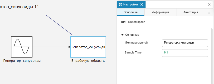
In addition to the software decimation methods mentioned in section 1.5, it is also convenient to pre-use the standard block methods for lowering the sampling rate.:

by reducing the sampling rate in the ToWorkspace block,
using the [Rate Transition] block(https://engee.com/helpcenter/stable/en/base-lib-signal-attributes/rate-transition.html ) (Transition between sampling rates)

Reduced sampling rate (Sample time: -1 -> 0.1)

Transition between sampling rates:

Conclusion

Both presented methods allow you to organize the software processing of simulation results. In the first case, the ability to work with Julia programming constructs and knowledge of Engee programming entities are more required. In the second case, additional blocks must be installed for each recorded signal.

The determining factors here are the needs, competencies, and user convenience.

Row	time	value
	Float64	Float64
1	0.0	0.0
2	0.01	0.309017
3	0.02	0.587785
4	0.03	0.809017
5	0.04	0.951057
6	0.05	1.0
7	0.06	0.951057
8	0.07	0.809017
9	0.08	0.587785
10	0.09	0.309017
11	0.1	1.22465e-16
12	0.11	-0.309017
13	0.12	-0.587785
⋮	⋮	⋮
90	0.89	0.309017
91	0.9	1.10218e-15
92	0.91	-0.309017
93	0.92	-0.587785
94	0.93	-0.809017
95	0.94	-0.951057
96	0.95	-1.0
97	0.96	-0.951057
98	0.97	-0.809017
99	0.98	-0.587785
100	0.99	-0.309017
101	1.0	-1.22465e-15

Row	time	value
	Float64	Float64
1	0.0	0.0
2	0.01	0.425779
3	0.02	0.770513
4	0.03	0.968583
5	0.04	0.982287
6	0.05	0.809017
7	0.06	0.481754
8	0.07	0.0627905
9	0.08	-0.368125
10	0.09	-0.728969
11	0.1	-0.951057
12	0.11	-0.992115
13	0.12	-0.844328
⋮	⋮	⋮
90	0.89	0.992115
91	0.9	0.951057
92	0.91	0.728969
93	0.92	0.368125
94	0.93	-0.0627905
95	0.94	-0.481754
96	0.95	-0.809017
97	0.96	-0.982287
98	0.97	-0.968583
99	0.98	-0.770513
100	0.99	-0.425779
101	1.0	-1.71451e-15

Modeling data processing

Introduction

1. We use simout

1.1. Getting a variable

1.2. Variable processing simout

1.3. Vector signal in value

1.4. Unnamed signal

1.5. Thinning

2. We use the To Workspace blocks

2.1. Getting variables

2.2. Processing variables

2.3 Thinning

Conclusion

1. We use `simout`

1.2. Variable processing `simout`

1.3. Vector signal in `value`