RC bandpass filter for frequency range selection
In this example, a passive bandpass RC filter is calculated and tested for a range of approximately 0.75 kHz to 16 kHz. The script shows the calculation of ratings, the construction of the expected amplitude-frequency response, the launch of ready-made Engee models and the comparison of the signal model with a physical electrical circuit.
Introduction
This example describes the progress of solving the problem.
2W1.2 - Bandwidth
from the book
** Thomas K. Hayes, Paul Horowitz
The Art of Circuit Engineering: Theory and Practice**
by computer simulation in Engee.
The task requires obtaining a filter that attenuates frequencies that are too low, skips the operating range, and weakens the high-frequency component again.
Practically, such a filter can be assembled from two simple RC links. The low-frequency boundary is set by the high-frequency link, and the high-frequency boundary is set by the low-frequency link. It is important to choose the resistances so that the next cascade does not overload the previous one.
Theoretical background
A transfer function is used for the low-frequency link of the first order
For the first-order high-frequency link:
If we consider the cascades to be weakly coupled in terms of load, the bandpass filter describes the product:
The boundary frequencies of each RC link are estimated as
In the physical model, the output resistor of the upper frequency link has a resistance of 1 mOhm. Therefore, it is useful to consider the equivalent resistance for the lower bound.:
Calculation of parameters
In this cell, set the cascade resistances, target frequencies, and standard capacitances. Then compare the calculated border frequencies with the required range.
R_LP = 10_000.0
C_LP = 1e-9
R_HP = 100_000.0
C_HP = 2e-9
R_load = 1_000_000.0

f_low_target = 750.0
f_high_target = 16_000.0

parallel(R1, R2) = 1 / (1 / R1 + 1 / R2)
R_HP_loaded = parallel(R_HP, R_load)

f_lp = 1 / (2pi * R_LP * C_LP)
f_hp_ideal = 1 / (2pi * R_HP * C_HP)
f_hp_loaded = 1 / (2pi * R_HP_loaded * C_HP)

C_LP_exact = 1 / (2pi * f_high_target * R_LP)
C_HP_exact = 1 / (2pi * f_low_target * R_HP)

calculation_summary = (;
    R_LP,
    C_LP,
    f_lp,
    R_HP,
    C_HP,
    f_hp_ideal,
    R_HP_loaded,
    f_hp_loaded,
    C_LP_exact,
    C_HP_exact,
)

calculation_summary
The nominal value 1 nF for the low-frequency link gives an upper bound of about 15.9 kHz. The nominal value 2 nF for the high-frequency link gives a lower limit of about 796 Hz without load and about 875 Hz at load 1 mOhm. For an educational RC filter, this is close to the required band.
Description of models
Two Engee models have been prepared for testing.
RCBandPass_2W_1_2_signal.engee— signal model with blocksTransfer Fcn. It compares the ideal cascade transfer function and approximation with a load of 1 mOhm.RCBandPass_2W_1_2_phys.engee— the physical acausal model. In it, the voltage source feeds the RC circuit: first there is a low-frequency link 10 kOhm + 1 nF, then a high-frequency link 2 nF + 100 kOhm, and a load 1 mOhm is connected to the output.
The sum of three sinusoids is applied to the input: low frequency 200 Hz, frequency in the band 3 kHz and high frequency 30 kHz. This signal helps to see which components the filter suppresses and which it skips.
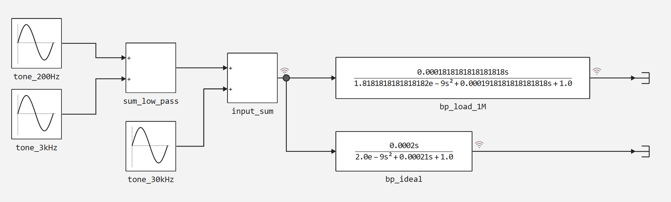
.png)
Environment preparation
In this cell, specify the paths to the finished models and the folder for the result files. If you are running the example from another directory, change the dir variable.
using Plots

dir = @__DIR__
output_dir = dir
model_paths = Dict(
    :signal => joinpath(dir, "RCBandPass_2W_1_2_signal.engee"),
    :physical => joinpath(dir, "RCBandPass_2W_1_2_phys.engee"),
)
string("prepared; dir=", dir)
The environment is ready: the models are next to the script, and the new graphs and tables will be saved to the same folder.
Analytical verification
Before running the models, build the calculated amplitude-frequency response. It shows the expected bandwidth and the effect of the load on the lower bound.
freqs = exp10.(range(log10(10.0), log10(100_000.0), length = 800))

gain_bp(f, R_hp) = begin
    tau_lp = R_LP * C_LP
    tau_hp = R_hp * C_HP
    omega = 2pi * f
    (omega * tau_hp) / sqrt((1 + (omega * tau_hp)^2) * (1 + (omega * tau_lp)^2))
end

p_response = plot(
    freqs,
    20 .* log10.(gain_bp.(freqs, R_HP));
    xscale = :log10,
    label = "no load",
    xlabel = "Frequency, Hz",
    ylabel = "Amplitude, dB",
    title = "Estimated frequency response of the RC bandpass filter",
)
plot!(p_response, freqs, 20 .* log10.(gain_bp.(freqs, R_HP_loaded)); label = "Rh = 1 mOhm")
vline!(p_response, [750.0, 16_000.0]; label = "task boundaries", linestyle = :dash)
hline!(p_response, [-3.0]; label = "-3 dB", linestyle = :dot)

response_path = joinpath(output_dir, "rc_bandpass_response.png")
savefig(p_response, response_path)
p_response
The graph shows the rise of the characteristic after the lower boundary and the decline after the upper boundary. The load 1 mOhm slightly shifts the lower limit upwards, because it simultaneously reduces the resistance of the output arm of the high-frequency cascade.
Simulation of the model
Now download the signal model and run the simulation. The code uses software management by Engee: engee.load, engee.open, engee.run and engee.close.
missing_models = [path for path in values(model_paths) if !isfile(path)]

if isempty(missing_models)
    signal_payload = Core.eval(Main, quote
        model = engee.load($(model_paths[:signal]); force = true)
        engee.open(model)
        results = engee.run(model)
        engee.close(model; force = true)
        (; results, result_text = repr(results))
    end)

    signal_results = signal_payload.results
    string("signal model simulated; results=", signal_payload.result_text)
else
    string("missing_models=", join(missing_models, ";"))
end
The signal model returns the input signal, the output of the ideal bandpass filter, and the output of the approximation with a load of 1 mOhm.
Checking the physical model
Run the physical model. It tests the same idea as an electrical circuit with a voltage source, resistors, capacitors, electric ground, voltage sensor, and block Solver Configuration.
physical_payload = Core.eval(Main, quote
    model = engee.load($(model_paths[:physical]); force = true)
    engee.open(model)
    results = engee.run(model)
    engee.close(model; force = true)
    (; results, result_text = repr(results))
end)

physical_results = physical_payload.results
string("physical model simulated; results=", physical_payload.result_text)
The physical model was completed successfully: the output voltage is recorded by the sensor.
Analysis of simulation results
Build time graphs of the signal model. They show how, out of the sum of the three harmonics of the signal, there remains mainly a component in the bandwidth.
function series_from_result(results, key)
    df = results[key]
    return df.time, df.value
end

time, input_signal = series_from_result(signal_results, "input_sum.1")
_, y_ideal = series_from_result(signal_results, "bp_ideal.1")
_, y_load = series_from_result(signal_results, "bp_load_1M.1")

p_time = plot(
    time .* 1000,
    input_signal;
    label = "entrance",
    xlabel = "Time, ms",
    ylabel = "Voltage, relative units",
    title = "Filtering the sum of three tones",
)
plot!(p_time, time .* 1000, y_ideal; label = "the perfect cascade model")
plot!(p_time, time .* 1000, y_load; label = "with a load of 1 mOhm")

time_plot_path = joinpath(output_dir, "rc_bandpass_time_signals.png")
savefig(p_time, time_plot_path)
p_time
The output is less influenced by the slow component 200 Hz and the high-frequency component 30 kHz. The signal in the range of 3 kHz passes better than the others, so the shape becomes closer to the midrange harmonic.
Comparison with a physical circuit
Build the input and output of the physical model. This graph is needed to make sure that the physical circuit behaves like a calculated bandpass filter.
time_phys, input_phys = series_from_result(physical_results, "input_sum.1")
_, vout_phys = series_from_result(physical_results, "vout_sensor.V")

p_phys = plot(
    time_phys .* 1000,
    input_phys;
    label = "physical model input",
    xlabel = "Time, ms",
    ylabel = "Voltage, V",
    title = "Checking the physical RC circuit",
)
plot!(p_phys, time_phys .* 1000, vout_phys; label = "output of the physical model")

physical_plot_path = joinpath(output_dir, "rc_bandpass_physical_time.png")
savefig(p_phys, physical_plot_path)
p_phys
The physical circuit also suppresses the low and high components. A slight difference from the ideal transfer function is expected: real cascades interact via impedances, and the output is additionally loaded with a resistance of 1 mOhm.
Summary table
Put the calculated indicators in a table. It records the band boundaries and transmission coefficients at the test frequencies.
case_rows = [
    (case = "ideal", R_hp = R_HP),
    (case = "load_1M", R_hp = R_HP_loaded),
]

summary_rows = [
    (;
        case = row.case,
        f_hp_Hz = 1 / (2pi * row.R_hp * C_HP),
        f_lp_Hz = f_lp,
        gain_200Hz = gain_bp(200.0, row.R_hp),
        gain_750Hz = gain_bp(750.0, row.R_hp),
        gain_3kHz = gain_bp(3_000.0, row.R_hp),
        gain_16kHz = gain_bp(16_000.0, row.R_hp),
        gain_30kHz = gain_bp(30_000.0, row.R_hp),
    )
    for row in case_rows
]

summary_csv = joinpath(output_dir, "rc_bandpass_summary.csv")
open(summary_csv, "w") do io
    println(io, "case,f_hp_Hz,f_lp_Hz,gain_200Hz,gain_750Hz,gain_3kHz,gain_16kHz,gain_30kHz")
    for row in summary_rows
        println(io, join((row.case, row.f_hp_Hz, row.f_lp_Hz, row.gain_200Hz, row.gain_750Hz, row.gain_3kHz, row.gain_16kHz, row.gain_30kHz), ","))
    end
end

summary_rows
The table confirms the engineering goal: the transmission coefficient of about 3 kHz is the highest among the selected test frequencies, and the frequencies 200 Hz and 30 kHz are noticeably weakened.
Conclusion
We calculated and tested the RC bandpass filter for a range of approximately 0.75 kHz to 16 kHz. The ratings 10 kOhm + 1 nF and 2 nF + 100 kOhm give close band boundaries, and the load 1 mOhm moderately shifts the lower boundary. The Engee signal and physical models consistently show the suppression of low and high components during the passage of a midrange signal.
List of literature
- Hayes T.K., Horowitz P. ** The art of circuit engineering. Theory and practice.** BHV-Petersburg, 2022. pp.130-132
- Horowitz P., Hill U. ** The art of circuit engineering.** Volume 1. Mir, 1993.
- Bessonov L. A. Theoretical foundations of electrical engineering. Electrical circuits. Gardariki, 2002.
- Sedra A., Smith K. Microelectronic circuits. Williams.
- Engee Help Center. Block documentation
Transfer Fcn,Sine Wave,Add,Resistor,Capacitor,Electrical Reference,Controlled Voltage Source,Voltage Sensor,Solver Configuration. - Engee Help Center. Software model management:
engee.load,engee.open,engee.run,engee.close.