Controlled thyristor T123-200 with cooler O123
This interactive script shows a method for developing and testing a model of a single-phase thyristor regulator with a T123-200 power thyristor and an O123 cooler. The material is useful for engineers and students who build physical models of power electronics at Engee and want to link the parameters of the blocks with the device's passport data, thermal calculation and pulse-phase control algorithm. Using the model example VT.engee The choice of the level of detail of the thyristor, the calculation of open-state losses, the selection of a thermal circuit, the justification of the RL load, RC protection circuit, decoupled gate control circuit and the SIFU subsystem are considered. The code cells perform control analytical calculations, run the model without changing the source file, and plot current, voltage, average values, and adjustment characteristics. The formulas and calculation procedure are based on the dataset and reference literature.
1. The methodology of model construction
The development of a power thyristor controller model does not begin with the choice of blocks, but with the choice of the physical boundary of the task. In the educational and engineering setting, it is convenient to divide the model into four parts: a power circuit, a control circuit, a synchronization and phase control system, and a thermal circuit. This separation repeats the structure of a real device: energy is transferred through the anode-cathode of the thyristor and the load, a control pulse is introduced through a separate low-power channel, and thermal power is removed from the semiconductor structure through the housing and radiator.
In Engee, a block is selected for the power thyristor Thyristor, not a perfect key. The reason is fundamental: the calculation requires a holding current, a control current and voltage, an open voltage drop, a thermal port and a tabular VAC. The ideal key is good for logical verification of the algorithm, but it does not provide correct losses and temperatures. Engee Documentation explicitly states that the block Thyristor It can be parameterized either by an equivalent transistor circuit or by an open-state VAC table; the table is more convenient for the passport model of an industrial device because it is closer to the graphs from the passport[8].
The power part is built as a controlled rectification on an inductive load. The inductance does not allow instantaneous current loss, so the model needs a free-pass branch with a diode. The RC circuit is placed parallel to the thyristor as a switching surge damper and as an element limiting the rate of voltage change. . The thermal port of the thyristor is connected to the radiator and the thermal mass of the medium.
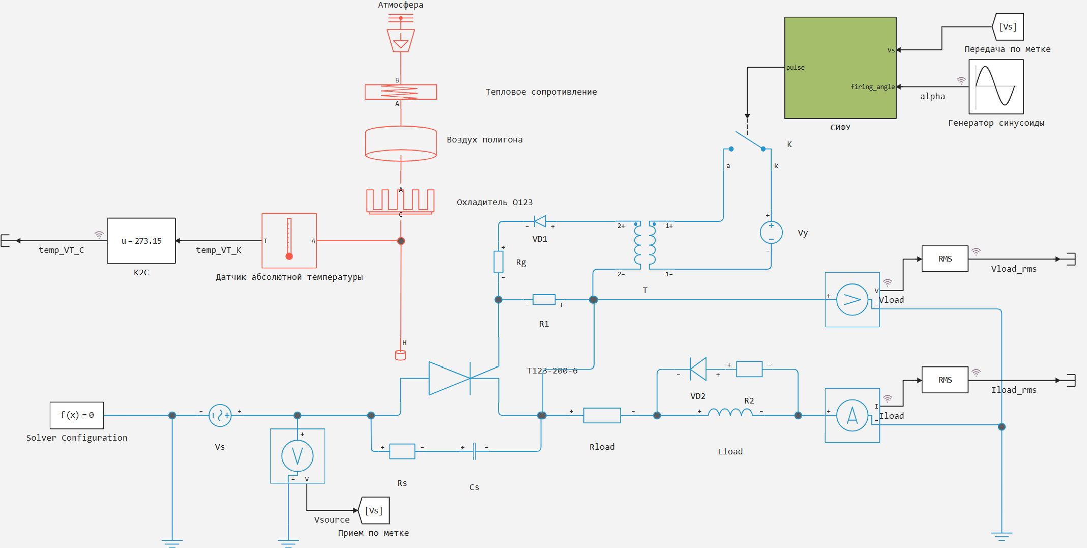
In this example, we will assemble the following schematic diagram: 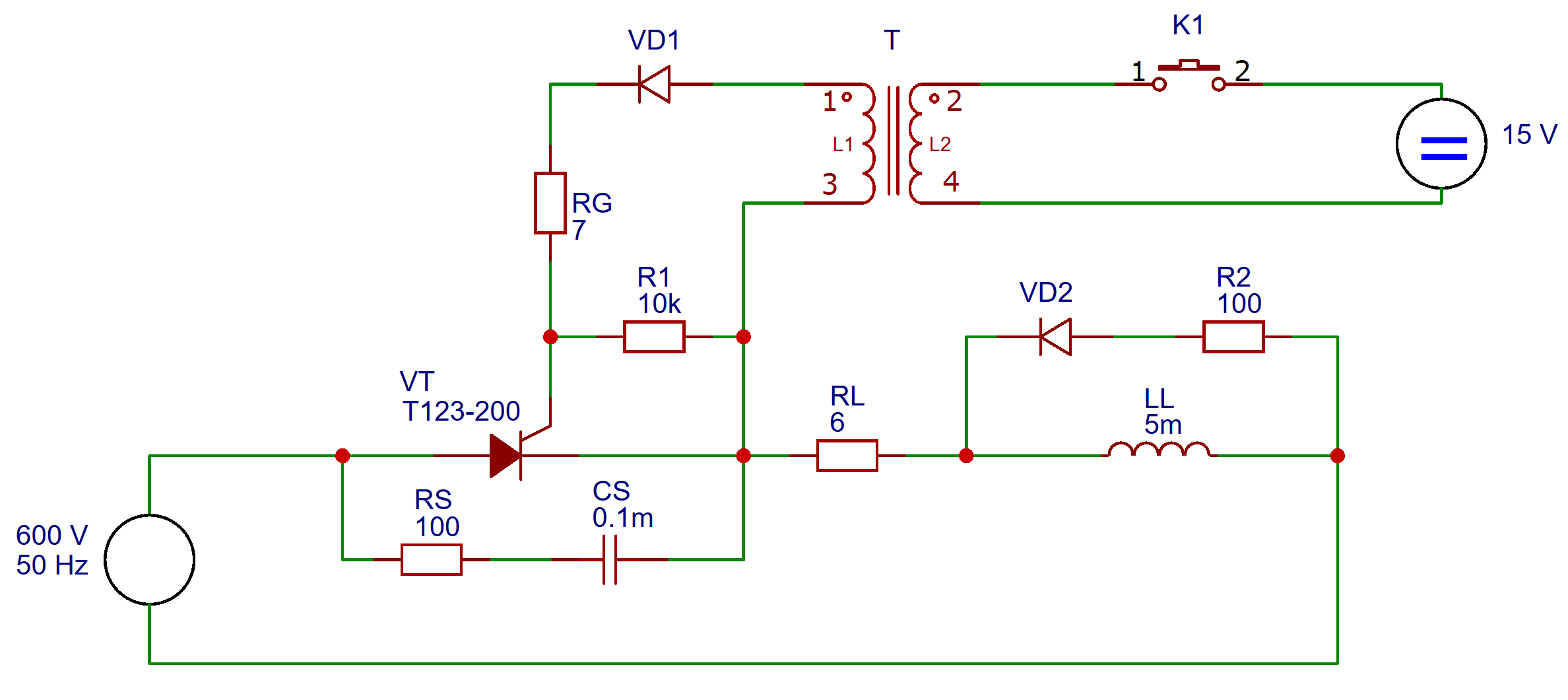
The key K1 is replaced here with an ideal semiconductor key. К, controlled from a pulse-phase control system.
2. From the passport of the thyristor to the block parameters
The passport data is first translated into a set of parameters that are actually used by the model. For T123-200, the calculation requires: a repetitive voltage class , average and current currents of the open state and , holding current , control parameters and , threshold voltage of the open state , dynamic resistance , the limiting temperature of the transition , thermal resistances and .
The voltage class is selected based on the maximum voltage on a closed thyristor with a margin. For the network the amplitude is equal to
Class 6 on it is not sufficient for such a network, so the model has , corresponding to the T123-200-16 version. This provides a margin for network peaks and recurring overvoltages.
The open state is set by a tabular dependency . The passport gives a graph of the VAX, therefore, you need to select several points from it and enter I_on_vector and V_on_vector. If only a linear approximation is available, use
This approximation is used in reference calculations of losses of power semiconductor devices; it is also given in Appendix C of GOST R IEC 61800-4-2012 for losses in an open thyristor[4].
3. Calculation of losses and control pulse
The average loss power in the open state is estimated by the average and effective current values:
The first term describes losses at a conditional threshold voltage drop, the second term describes ohmic losses at the internal resistance of the VAC. For the initial assessment, values are taken at the maximum transition temperature, because the thermal calculation must be conservative.
The control circuit must ensure that the current of the control electrode is higher than the rated current . In practical schemes, a reserve is laid because it depends on the temperature, the spread of the device and the shape of the pulse. This technique uses verification
For the source , unlocking voltage and consecutive resistances The estimated current is
It's higher .
Thus, in the model, the control pulse is supplied through a real electrical branch with a source, key, transformer, diode and resistors, rather than a direct logical signal in the control electrode circuit: this method preserves the physical meaning of the control current and takes into account the total resistance of the control electrode circuit[8].
4. Parameterization of the O123 thyristor radiator model
The radiator in the model is parameterized according to the passport. It is important not to replace the radiator with the usual constant thermal resistance if a dynamic thermal picture is required: the passport specifies the mass, material and thermal resistances, and the block Радиатор In Engee, you can set not only the static heat dissipation, but also the thermal capacity.
Basic passport data for O123:
| Parameter | Designation | Meaning |
|---|---|---|
| Rated power dissipation | ||
| Thermal resistance during natural cooling | ||
| Thermal resistance during forced cooling | ||
| Radiator weight | ||
| Specific heat capacity of aluminum alloy |
Dynamic characteristics
The mass of the radiator is taken directly from the passport: . The material is specified as a corrosion-resistant aluminum alloy, so the typical value can be accepted.
Heat sink capacity:
This parameter is needed for the transient thermal process.: More than the slower the radiator temperature increases with the same power dissipation.
Reference point of the steady state
The formula of thermal resistance:
Hence the temperature difference at rated power and natural convection:
This point is used as a reference point for building the block's tabular dependency. Радиатор: , .
A power-law model of natural convection
For natural air cooling, it is convenient to approximate the heat flow by a power dependence:
For natural convection, the indicator is taken . Ratio located from a reference point:
After that, the power output by the radiator at the selected temperature vector is calculated as
The model uses a vector . This set of points is convenient for tabular parameterization: it covers low, medium, and close to nominal radiator overheating without overloading the model with unnecessary points.
Alternative linear estimation
For control, you can compare a power-law model with a linear one.:
The linear model passes through the origin and assumes constant thermal resistance. The power model better reflects natural convection, where the intensity of heat transfer varies with overheating. Therefore, for the block Радиатор a tabular vector is used calculated according to the power law, and the linear estimate remains the control one.
#=
Parameterization of the radiator O123.
This cell repeats the calculation of the parameters that are entered into the Radiator block:
mass, specific heat capacity, temperature drop vector, and power output vector.
The power dependence is used for natural convection; the linear model is abandoned
as a benchmark for constant thermal resistance.
=#

using Printf

# Passport parameters of O123
P_nominal = 120.0      # power dissipation, W
Rth_natural = 0.71     # thermal resistance during natural cooling, °C/W
Rth_forced = 0.212     # thermal resistance during forced cooling, °C/W
mass = 2.0             # radiator weight, kg
cp_aluminum = 900.0    # specific heat capacity of aluminum alloy, J/(kg*K)

println("The main parameters of the radiator O123:")
println("Weight: $mass kg")
println("Specific heat capacity: $cp_aluminum J/(kg*K)")
println("Rated Power: $P_nominal W")
println("Thermal resistance, natural cooling: $Rth_natural °C/W")
println("Thermal resistance, forced cooling: $Rth_forced °C/W")

# Dynamic part of the model: the thermal capacity sets the inertia of heating.
heatsink_heat_capacity = mass * cp_aluminum

println()
println("=== DYNAMIC CHARACTERISTICS ===")
println("Radiator weight: ", mass, " kg")
println("Specific heat capacity: ", cp_aluminum, " J/(kg*K)")
println("Heat sink capacity: ", heatsink_heat_capacity, " J/K")

# Reference point for natural convection from rated power and Rth.
delta_T_nominal = P_nominal * Rth_natural

println()
println("=== CALCULATION OF THE REFERENCE POINT ===")
println("Rated power P = ", P_nominal, " Tue")
println("Thermal resistance Rth = ", Rth_natural, " °C/W")
println("Temperature difference ΔT = P * Rth = ", round(delta_T_nominal, digits=2), " K")
println("Reference point: (ΔT = ", round(delta_T_nominal, digits=2), " K, Q = ", P_nominal, " Tue)")

# For natural convection, we use the power law Q = k* ΔT^n.
n = 1.25
k = P_nominal / (delta_T_nominal^n)

println()
println("=== POWER DEPENDENCE PARAMETERS ===")
println("Exponent of n = ", n)
println("Coefficient k = ", round(k, digits=4))
println("Formula: Q = ", round(k, digits=4), " * ΔT^", n)

# The vector ΔT corresponds to the tabular parameterization of the radiator in the model.
delta_T_vector = [10.0, 30.0, 50.0, 70.0, 90.0]
Q_vector = [k * (dT^n) for dT in delta_T_vector]

println()
println("=== VECTORS FOR PARAMETERIZATION OF THE MODEL ===")
println("Temperature difference vector ΔT, K:")
println(delta_T_vector)
println("Vector of output power Q, W:")
println(round.(Q_vector, digits=1))
println()
println("Table of values:")
println("│ ΔT, K │ Q, W │")
println("├───────┼─────────┤")
for (i, dT) in enumerate(delta_T_vector)
    @printf("│ %6.1f │ %7.1f │\n", dT, Q_vector[i])
end

# Verification: At the reference point, the power model should return P_nominal.
Q_check = k * (delta_T_nominal^n)
error = abs(Q_check - P_nominal)

println()
println("=== CHECKING THE CALCULATION ===")
println("At ΔT = ", round(delta_T_nominal, digits=2), " K:")
println("  Estimated power Q = ", round(Q_check, digits=2), " Tue")
println("  Rated power = ", P_nominal, " Tue")
println("  Error rate = ", round(error, digits=4), " Tue")

println()
println("="^60)
println("SUMMARY PARAMETERS FOR THE MODEL")
println("="^60)
println("Parameterization method: tabular dependence Q(ΔT)")
println("Type of convection: natural")
println("Vector ΔT, K: [", join(round.(delta_T_vector, digits=1), ", "), "]")
println("Vector Q, W: [", join(round.(Q_vector, digits=1), ", "), "]")
println("Radiator weight: ", mass, " kg")
println("Specific heat capacity: ", cp_aluminum, " J/(kg*K)")

# The linear model is only needed for comparison with nonlinear natural convection.
Q_linear = [dT / Rth_natural for dT in delta_T_vector]

println()
println("=== LINEAR MODEL FOR COMPARISON ===")
println("Thermal resistance Rth = ", Rth_natural, " °C/W")
println("Vector Q of the linear model, W:")
println(round.(Q_linear, digits=1))
println()
println("│ ΔT, K │ Q power law, W │ Q linear, W │")
println("├───────┼─────────────────┼────────────────┤")
for (i, dT) in enumerate(delta_T_vector)
    @printf("│ %6.1f │ %15.1f │ %14.1f │\n", dT, Q_vector[i], Q_linear[i])
end

string(
    "Cth=", round(heatsink_heat_capacity; digits=1),
    " J/K; delta_T_nom=", round(delta_T_nominal; digits=2),
    " K; Q_vector=", join(round.(Q_vector; digits=1), ","),
)
5. Calculation of electrical and control units
The network source is set by the amplitude, not the current value.:
By the period is equal to
The RL load is needed to demonstrate a mode with current continuity and phase shift. Its parameters are estimated through the inductive resistance, the impedance modulus and the electromagnetic time constant:
For and we get , , . This time constant characterizes the dynamics of the transient process in the load circuit. A freewheel diode (reverse diode) with a series-connected resistance is needed to protect the power circuit from damage caused by a sudden change in current in the inductive load when the thyristor is closed.
The RC circuit has a time constant
This circuit sets the damping path for dynamic processes in the thyristor circuit.
The thermal mass of the air is calculated using the formula
This one may be needed to simulate the inertia of the polygon environment.
6. Pulse-phase control system
The SIFU is built as a synchronized delay from the transition of the mains voltage through zero. Block Пересечение уровня highlights the beginning of the half-cycle, RS-триггер generates a logical signal with a duration of , defined by the block Транспортное запаздывание, and Переменное временное запаздывание transfers the release moment to the value set by the control angle.
Setting the angle in the model:
Limiter Насыщение sets the acceptable range . For the current sine wave, the actual range is Therefore, the lower limit does not distort the signal, but protects the model at a different assignment amplitude. The relationship between angle and delay:
By this gives a range of delays . This structure was chosen instead of an arbitrary pulse generator because it retains the main property of phase control: the opening moment is always counted from the phase of the supply voltage, and not from an independent clock.
.png)
7. Analytical calculation before launching the model
The next code cell performs a control calculation of the passport, electrical and thermal values. The network amplitude, thyristor losses, total thermal resistances, transition temperature estimation, RL load parameters, RC circuits, SIPHON delay range and control current reserve are checked in the cell.
This cell does not access VT.engee it is needed as an engineering check of the initial numbers before numerical modeling.
#=
Only analytical estimates are collected here. Their goal is to check quickly.,
that the passport data and block parameters are agreed upon before launching the model.
The formulas themselves are included in the text above, and numerical substitutions are left below.
=#

# Calculation of passport and model parameters
using Printf

f = 50.0
T = 1 / f
U_rms = 600.0
U_peak = sqrt(2) * U_rms

ITAVM = 200.0
ITRMS = 315.0
UT0 = 1.05
rT = 1.17e-3
P_TAV = UT0 * ITAVM + rT * ITRMS^2

Rth_jc = 0.080
Rth_ch = 0.020
Rth_ha_nat = 0.710
Rth_ha_forced = 0.212
Rth_ja_nat = Rth_jc + Rth_ch + Rth_ha_nat
Rth_ja_forced = Rth_jc + Rth_ch + Rth_ha_forced

T_ambient = 25.0
Tj_est_nat = T_ambient + P_TAV * Rth_ja_nat
Tj_est_forced = T_ambient + P_TAV * Rth_ja_forced

R_load = 6.0
L_load = 5e-3
X_L = 2*pi*f*L_load
Z_load = sqrt(R_load^2 + X_L^2)
tau_load = L_load / R_load

Rs = 100.0
Cs = 1e-4
tau_snubber = Rs * Cs

alpha_min = 90.0 - 82.0
alpha_max = 90.0 + 82.0
delay_min = alpha_min * T / 360
delay_max = alpha_max * T / 360

Vgate_source = 15.0
VGT = 3.5
IGT = 0.20
R2 = 7.0
Rg = 10.0
Ig_est = (Vgate_source - VGT) / (R2 + Rg)

rows = [
    ("Network period T", T, "with"),
    ("Vm Network Amplitude", U_peak, "In"),
    ("Thyristor losses at ITAVM/ITRMS", P_TAV, "Tue"),
    ("Rthja is natural", Rth_ja_nat, "K/W"),
    ("Rthja forced", Rth_ja_forced, "K/W"),
    ("Tj rating under natural cooling", Tj_est_nat, "°C"),
    ("Tj rating for forced cooling", Tj_est_forced, "°C"),
    ("Load inductive resistance XL", X_L, "Om"),
    ("Load impedance module |Z|", Z_load, "Om"),
    ("Load time constant L/R", tau_load, "with"),
    ("RC Circuit time constant", tau_snubber, "with"),
    ("Minimum SIFU delay", delay_min, "with"),
    ("Maximum SIFU delay", delay_max, "with"),
    ("Gate control current estimation", Ig_est, "But"),
    ("Stock to 3*IGT", Ig_est / (3*IGT), "once"),
]

for (name, value, unit) in rows
    @printf("%-46s = %12.6g %s\n", name, value, unit)
end

string("U_peak=", round(U_peak; digits=2), " V; P_TAV=", round(P_TAV; digits=2), " W; Ig/(3IGT)=", round(Ig_est/(3IGT); digits=3))
8. Program launch of the model and data preparation
The next code cell loads the existing model VT.engee, temporarily limits the calculation time in an open session, enables logging of the necessary ports, starts modeling and converts the results into arrays for graphs.
Limitation StopTime before It was introduced for practical reasons, since a fixed step is set in the model. and a large number of points received will negatively affect the convenience of interacting with the model.
#=
Launching the model.
This cell performs three tasks: it prepares the environment.,
runs the existing Engee model and converts the results to arrays.
=#

include("$(@__DIR__)/useful_functions.jl")

# Before uploading, we close the model of the same name so as not to mix the results of different launches.

try_close_model(model_name)
model_path = resolve_existing_file(model_file)
model = engee.load(model_path; force=true)
engee.open(model)

# We remember the initial settings only for the report in the status bar.

original_stop_time = safe_model_param(model, "StopTime", "")
original_fixed_step = safe_model_param(model, "FixedStep", "")
original_solver = safe_model_param(model, "SolverName", "")

status_message = ""

# The time limit of the calculation in the current session. The model file is not saved.
safe_set_model_param!(model, "StopTime", string(simulation_stop_time))

# Temporary recording of signals in the current session. The original model file is not saved.
log_ports = [
    "Sinusoid generator/1",
    "Voltage sensor/1",
    "Current sensor/1",
    "Offset/1", # temperature of the heating unit after conversion from K to °C
]

for port in log_ports
    safe_set_log(port)
end

# We run the model after configuring logging; the Engee result is read as a set of named signals.

results = engee.run(model)

# We extract three key signals: opening angle, load voltage and load current.

(angle_xy, angle_key) = get_signal(results, ["alpha", "The sine wave generator.1", "The sine wave generator.main_out", "The sine wave generator"])
(vload_xy, vload_key) = get_signal(results, ["Vload", "The voltage sensor.Vload", "The voltage sensor.1", "The voltage sensor.v_out"])
(iload_xy, iload_key) = get_signal(results, ["Iload", "Current sensor.Iload", "Current sensor.1", "Current sensor.i_out"])

# We thin the instantaneous signals to 1000 points before visualization.

t_alpha, alpha = thin(angle_xy[1], angle_xy[2]; max_points=max_plot_points)
t_v, vload = thin(vload_xy[1], vload_xy[2]; max_points=max_plot_points)
t_i, iload = thin(iload_xy[1], iload_xy[2]; max_points=max_plot_points)

# We calculate the average values for one network period and also thin out the result.

v_avg_full = moving_average_by_time(vload_xy[1], vload_xy[2], network_period)
i_avg_full = moving_average_by_time(iload_xy[1], iload_xy[2], network_period)
t_vavg, v_avg = thin(vload_xy[1], v_avg_full; max_points=max_plot_points)
t_iavg, i_avg = thin(iload_xy[1], i_avg_full; max_points=max_plot_points)

try_close_model(model_name)
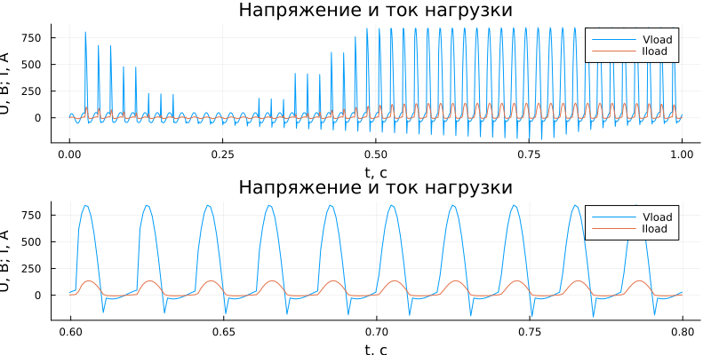
9. Current and voltage waveforms
The following code cell plots two basic graphs: the instantaneous load voltage and the instantaneous load current. Using these oscillograms, it is checked that the thyristor opens with a phase delay, the inductive load current does not stop instantly, and the amplitudes are in the expected range.
# This cell shows the instantaneous waveforms after the phase control.
p1 = plot(t_v, [vload, iload]; label=["Vload" "Iload"], xlabel="t, with", ylabel="U, B; I, A", title="Load voltage and current", legend=:topright, size=(800, 400))
period = 600:800
p2 = plot(t_v[period], [vload[period], iload[period]]; label=["Vload" "Iload"], xlabel="t, with", ylabel="U, B; I, A", title="Load voltage and current", legend=:topright, size=(800, 400))
plot(p1, p2; layout=(2, 1), size=(800, 400))
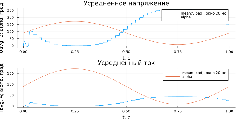
10. Comparison of the average values with the opening angle
The next code cell compares the voltage and current averaged over the period of the network with the signal of the opening angle . The averaging is performed in the previous cell of the sliding window simulation , that is , for one period of the network . Such a graph does not show individual switching edges, but a slow adjustment reaction of the load to a change in angle.
# Here, the average values for the period are compared with a slowly changing opening angle.

p3 = plot(t_vavg, [v_avg, alpha]; label=["mean(Vload), 20 ms window" "alpha"], xlabel="t, with", ylabel="Uavg, In; alpha, deg", title="Average voltage", legend=:topright)
p4 = plot(t_iavg, [i_avg, alpha]; label=["mean(Iload), 20 ms window" "alpha"], xlabel="t, with", ylabel="Iavg, A; alpha, deg", title="Average current", legend=:topright)
plot(p3, p4; layout=(2, 1), size=(800, 400))
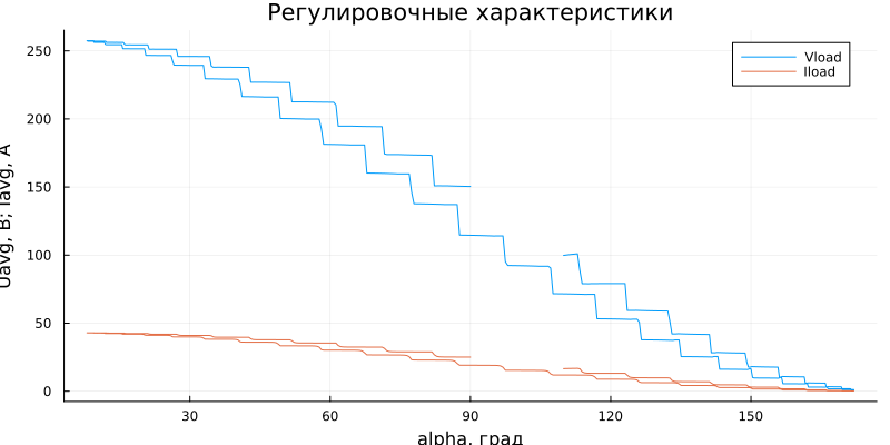
11. Adjustment characteristic
The next code cell plots the dependence of the average output values on the opening angle. The starting points are discarded by the index 40:end to reduce the impact of the transient at the beginning of the calculation. This graph is convenient for engineering output: when increasing The average voltage and current of the controlled rectifier decrease, and when the angle decreases, they increase.
# The graph in alpha coordinates shows the load adjustment characteristic.

plot(alpha[40:end], [v_avg[40:end], i_avg[40:end]]; label=["Vload" "Iload"], xlabel="alpha, hail", ylabel="Uavg, B; Iavg, A", title="Adjustment characteristics", legend=:topright, size=(800, 400))
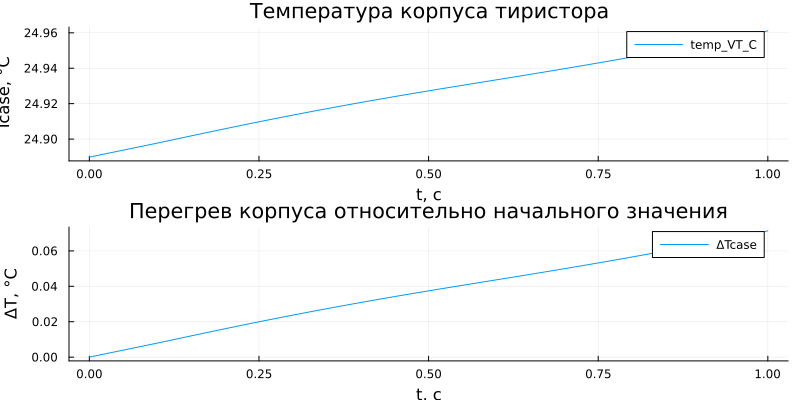
12. Temperature of the thyristor housing
In the thermal part of the model, the absolute temperature sensor is connected to the thermal node of the thyristor and radiator, and the unit Смещение converts the result from Kelvin to degrees Celsius. Therefore, the graph below should be read as the temperature of the housing/contact heat node, and not as the temperature of the crystal. The connection is used to estimate the transition temperature
Here It is taken from the simulation, - the thermal power dissipated by the thyristor, - rated thermal resistance of the junction housing. If it is the transition temperature that is required, the corresponding internal thermal output is added to the model or calculated after calculation through losses and .
The next code cell extracts the temperature signal from the simulation results, limits the number of points to max_plot_points and it plots two curves: the absolute temperature of the housing and overheating relative to the initial value. On a short interval the graph usually grows slowly because the radiator O123 has a large thermal capacity . Such a result is physically expected: electrical processes are established in milliseconds, and the thermal process develops over a much longer period of time.
# This cell extracts and plots the temperature of the thyristor housing/heat node.
# The list of names has been left expanded because Engee can return the signal by the name of the line.,
# the block name or the automatically generated port name.
(temp_xy, temp_key) = get_signal(results, [
    "temp_VT_C",
    "tempC",
    "Offset.temp_C",
    "Offset.1",
    "Offset.main_out",
    "Absolute temperature sensor.1",
])

t_temp, temp_case = thin(temp_xy[1], temp_xy[2]; max_points=max_plot_points)
temp_rise = temp_case .- first(temp_case)

p_temp1 = plot(
    t_temp,
    temp_case;
    label=temp_key,
    xlabel="t, with",
    ylabel="Tcase, °C",
    title="Temperature of the thyristor housing",
    legend=:topright,
)

p_temp2 = plot(
    t_temp,
    temp_rise;
    label="ΔTcase",
    xlabel="t, with",
    ylabel="ΔT, °C",
    title="Overheating of the housing relative to the initial value",
    legend=:topright,
)

plot(p_temp1, p_temp2; layout=(2, 1), size=(800, 400))
Bibliographic list and reference sources
- Rozanov Yu. K., Ryabchitsky M. V., Kvasnyuk A. A. [Power electronics: textbook for universities](https://www.studentlibrary.ru/book/ISBN9785383010235.html Moscow: MEI Publishing House, 2016.
- Chizhenko I. M., Rudenko V. S., Senko V. I. Fundamentals of transformational техники.
- Herman-Galkin S. G. [Computer simulation of semiconductor systems in MATLAB 6.0] (https://myebooks.narod.ru/german/index.htm ). St. Petersburg: KORONA print, 2001.
- GOST R IEC 61800-4-2012. Speed-controlled electric drive systems.
- Grebennikov V. V. Study of characteristics тиристоров
- SEMIKRON Danfoss. Application Manual Power Semiconductors.
- Engee. Software Script Management.
- Engee. Thyristor.
- Engee. Radiator.
- Passport
Тиристор T123-200 datasheet.pdf. - Passport
Охладитель О123 datasheet.pdf.