Simulation of an LVDT sensor in a one-dimensional setting
A Linearly Adjustable Differential Transformer (LVDT - Linear Variable Differential Transformer) is an electromechanical converter that converts linear motion of an object into an alternating current electrical signal. Structurally, the sensor consists of one primary winding, two identical secondary windings and a movable ferromagnetic core (rod).
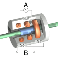
General view of the model
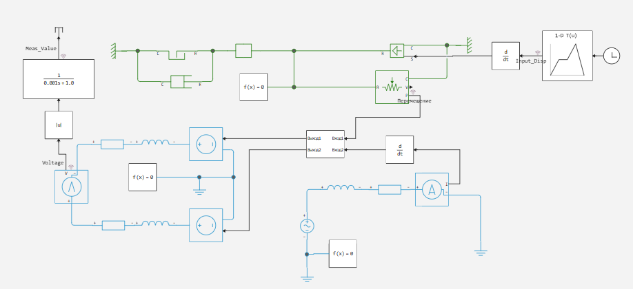
The core (above) moves according to an arbitrary law inside the primary (right, bottom) and secondary windings (left).
The physical law of induction
When an alternating voltage is applied to the primary winding, an alternating magnetic field arises around it, inducing an electromotive force. (EMF) in secondary windings based on Faraday's law of electromagnetic induction:
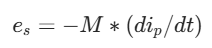
where e_s is the induced EMF in the secondary winding, i_p is the instantaneous current in the primary circuit, and M is the mutual inductance between the windings, depending on the geometry and position of the core.
Differential principle and balance of inductors
The LVDT secondary windings are wound symmetrically and connected in series (differentially). This means that the resulting voltage at the sensor output is equal to the voltage difference between the two secondary windings.:
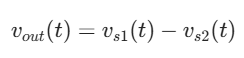
When the ferromagnetic core is located strictly in the center (in the zero position, x = 0), the magnetic fluxes penetrating both secondary coils are equal. Accordingly, their mutual inductors are equal.:
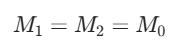
In this position, the induced voltages completely cancel each other, and the difference signal is zero. This state is called the electrical zero of the sensor.
When the core is shifted by an amount of x, the overlap area of the coils changes linearly, which leads to a proportional change in the mutual inductance coefficients.*:
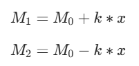
where k is the sensitivity coefficient (steepness of the coupling), expressed in Henry per meter (Gn/m) or Henry per millimeter (Gn/mm).
*In one-dimensional physical models, there is no finite element calculation of the distribution of magnetic fields in space. For this reason, the mutual influence of contours is described analytically through the phenomenological coefficients M(x). The accepted assumption of a strictly linear change in inductors The x coordinate is valid for the sensor's working area (x<= ±10 mm), since the scattering flux is minimal in it, and the volume of the ferromagnetic core penetrating each of the secondary coils varies in direct proportion to the movement of the rod.
Calculation of secondary winding voltages
Instead of using standard passive transformers, secondary windings are modeled using controlled EMF sources (Controlled Voltage Source). The voltages for controlling these sources are calculated dynamically at each integration step based on Faraday's law and the obtained analytical coupling coefficients.:

The calculation of the secondary winding voltages in the model is performed in the subsystem block:
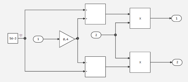
Let's open the model and plot the sensor measurements.
modelName = "LVDT"
if !(modelName in [m.name for m in engee.get_all_models()]) engee.load( "$(@__DIR__)/$(modelName).engee"); end;
data = engee.run( modelName )
# 1. Extracting the source data
Meas_Value = vec(collect(WorkspaceArray{Float64}("$modelName/Meas_Value")).value)
Input_Disp = vec(collect(WorkspaceArray{Float64}("$modelName/Input_Disp")).value)
Voltage = vec(collect(WorkspaceArray{Float64}("$modelName/Voltage")).value)
time_raw = collect(WorkspaceArray{Float64}("$modelName/Input_Disp")).time

# 2. Calculation of the thinning step for general graphs (p1, p2, p3)
target_dt = 0.0001
initial_dt = time_raw[2] - time_raw[1] # Fixed the definition of the time step
step_size = round(Int, target_dt / initial_dt)

if step_size < 1
    step_size = 1
end

# 3. Thinning for overview charts
time_ds = time_raw[1:step_size:end]
Input_Disp_ds = Input_Disp[1:step_size:end]
Voltage_ds = Voltage[1:step_size:end]
Meas_Value_ds = Meas_Value[1:step_size:end]

# 4. Charting
# We build general graphs based on thinned data (_ds)
p1 = plot( time_ds, Input_Disp_ds, title= "Core displacement, m")
p2 = plot( time_ds, Voltage_ds, title="Unfiltered voltage, V", linecolor = :orange)
p3 = plot( time_ds, Meas_Value_ds, title="Measured voltage, V", linecolor = :red)

# The p4 graph (zoom) is based on the initial data (time_raw, Voltage) without thinning
p4 = plot( time_raw, Voltage, title="Unfiltered voltage (zoom), V", linecolor = :green, xlims =(1, 1.001))

# The layout
plot( p1, p2, p3, p4, layout=(2,2), leg=false, size=(1200,600), titlefont=font(10) )
Conclusion
The one-dimensional physical model of the LVDT sensor developed in the Engee environment fully confirmed the theoretical laws of electromagnetic transformation. Dividing the model into a physical winding circuit and mathematical calculation of the EMF based on a real current change (di/dt) made it possible to create a flexible tool for designing automatic control systems and precision positioning, without the need for heavy FEM packages at the initial stages of development.