Numerical modeling of physical systems

This material is a set of demonstration examples designed to illustrate the capabilities of Engee and its ecosystem in solving problems of classical and modern physics. The main goal is to show how, using simple and expressive code, it is possible to simulate the dynamics of mechanical and electrodynamic systems, observe their behavior over time and visualize the results in the form of graphs and animations.

We will consider five key tasks: ballistics, harmonic oscillator with attenuation, motion of a charged particle in a constant magnetic field, nonlinear pendulum, double pendulum.

Each example is accompanied by a numerical solution of a system of ordinary differential equations (ODES) and animation (or static graph), which helps visualize physical processes.

try
    using DifferentialEquations
catch
    Pkg.add(["DifferentialEquations"])
    using DifferentialEquations
end

Paket DifferentialEquations.jl is a powerful library for solving differential equations developed within the framework of the SciML (Scientific Machine Learning) ecosystem. This library provides:

Wide range of solvers: from classical Runge–Kutta methods (Tsit5(), Vern7()) to specialized algorithms for rigid systems, differential algebraic equations, stochastic and delayed differential equations.
Flexible step control: solvers automatically select the integration step to achieve the specified accuracy, which frees the user from manual configuration.
Event mechanism (callbacks): allows you to stop integration when certain conditions are met (for example, touching the ground in ballistics) or to change parameters during the calculation process.
Convenient saving of results: parameter saveat It allows you to capture a decision at pre-set points in time, which is crucial for building smooth animations.

The work with the library is based on a single scheme:

Description of the ODE system in the form of a function returning derivatives (du).
Setting the initial conditions and the time interval.
Creating a task (ODEProblem) and its solution using the selected solver.
Processing and visualization of the resulting solution.

Ballistics

This example simulates the motion of a material point thrown at an angle to the horizon with an initial velocity in the gravity field. This is a classic problem of school and university physics, which clearly illustrates the basic principles of kinematics and dynamics. In our case, we consider an idealized case without air resistance, which allows us to obtain a parabolic trajectory and use an event mechanism to accurately determine the moment of falling to the ground.

Motion is described by a system of 4 first-order ODES for coordinates and velocities:

The initial conditions are set by the velocity modulus and the angle . Integration is carried out until the moment of touching the ground ().

The package is being used DifferentialEquations.jl:

The Solver: Tsit5() (adaptive Runge–Kutta method of the 5th order).
Events (Callbacks): Applied ContinuousCallback to accurately determine the moment of intersection . This stops the integration (terminate!) exactly at the moment of the fall, excluding errors of the discrete grid.
Visualization: A trajectory graph is created with marked and labeled key points: start, maximum, and drop location.

g = 9.81
v0 = 20.0
angle = deg2rad(45)
t_flight = 2 * v0 * sin(angle) / g  
tspan = (0.0, t_flight)
u0 = [0.0, 0.0, v0*cos(angle), v0*sin(angle)]

function ballistic!(du, u, p, t)
    du[1] = u[3]
    du[2] = u[4]
    du[3] = 0.0
    du[4] = -g
end

prob = ODEProblem(ballistic!, u0, tspan)
sol = solve(prob, Tsit5())

y_vals = sol[2, :]
idx_max = argmax(y_vals)

x_max = sol[1, idx_max]
y_max = y_vals[idx_max]
x_start, y_start = sol[1, 1], sol[2, 1]
x_end,   y_end   = sol[1, end], sol[2, end]

plot(sol[1, :], sol[2, :], label="The trajectory", lw=2,
     xlabel="x (m)", ylabel="y (m)", title="Ballistics",
     legend=:topright)

scatter!([x_start], [y_start], color=:blue,  markersize=8, label="Start")
scatter!([x_max],   [y_max],   color=:green, markersize=8, label="Max. height")
scatter!([x_end],   [y_end],   color=:red,   markersize=8, label="Fall")

annotate!(x_start, y_start - 0.5, text("Старт", :blue, 10))
annotate!(x_max,   y_max   + 0.5, text("Макс. высота", :green, 10))
annotate!(x_end,   y_end   - 0.5, text("Падение", :red, 10))

Harmonic oscillations of a spring pendulum

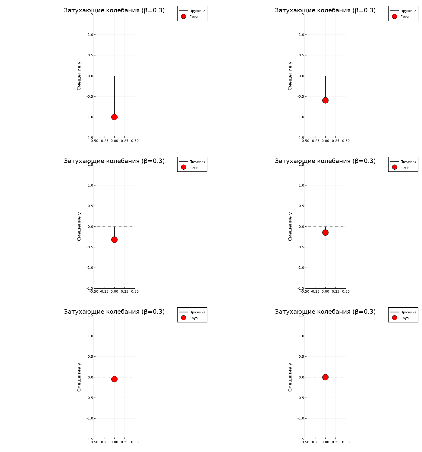
Next, damped oscillations of a spring pendulum are modeled. Motion is described by a system of 2 first-order ODES for displacement and speed :

where — natural frequency, — attenuation coefficient. Initial conditions: , .

This example expands the understanding of oscillators and shows how simple changes in the model (adding attenuation) qualitatively change the behavior of the system.

ω = 2.0
β = 0.3
A = 1.0
tspan = (0.0, 15.0)

u0 = [A, 0.0]

function harmonic_damped!(du, u, p, t)
    du[1] = u[2]
    du[2] = -ω^2 * u[1] - β * u[2]
end

prob = ODEProblem(harmonic_damped!, u0, tspan)
sol = solve(prob, Tsit5(), saveat=0.02)

@gif for i in 1:2:length(sol.t)
    y = sol[1,i]
    plot([0, 0], [0, -y], color=:black, lw=2, label="Spring",
         xlims=(-0.5, 0.5), ylims=(-1.5, 1.5),
         aspect_ratio=:equal, title="Затухающие колебания (β=$β)",
         xlabel="", ylabel="The y offset")
    scatter!([0], [-y], color=:red, markersize=10, label="Cargo")
    hline!([0], color=:gray, linestyle=:dash, label="")
end

The motion of a particle in a constant magnetic field.

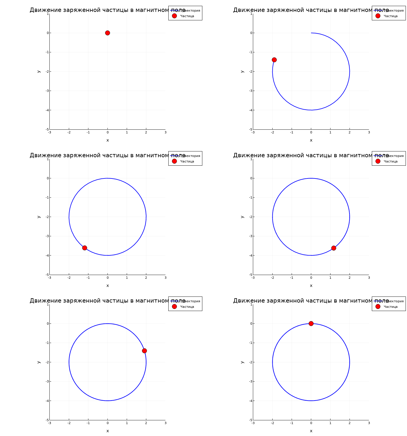
Now let's consider the motion of a charged particle in a uniform permanent magnetic field directed along the axis . Under the influence of the Lorentz force, the particle moves in a circle (cyclotron motion). The system is described by 4 first-order ODES for coordinates and velocities:

where — cyclotron frequency. Initial conditions: the particle starts from the origin with an initial velocity along the axis .

ω = 1.0
v0 = 2.0
tspan = (0.0, 2π/ω * 4)

u0 = [0.0, 0.0, v0, 0.0]

function lorentz!(du, u, p, t)
    du[1] = u[3]
    du[2] = u[4]
    du[3] = ω * u[4]
    du[4] = -ω * u[3]
end

prob = ODEProblem(lorentz!, u0, tspan)
sol = solve(prob, Tsit5(), saveat=0.02)

@gif for i in 1:length(sol.t)
    plot(sol[1, 1:i], sol[2, 1:i], 
         label="The trajectory", lw=2, color=:blue,
         xlabel="x", ylabel="y", 
         title="Motion of a charged particle in a magnetic field",
         aspect_ratio=:equal, 
         xlims=(-3, 3), ylims=(-5, 1))
    scatter!([sol[1,i]], [sol[2,i]], 
             color=:red, markersize=8, label="Particle")
end

The nonlinear pendulum

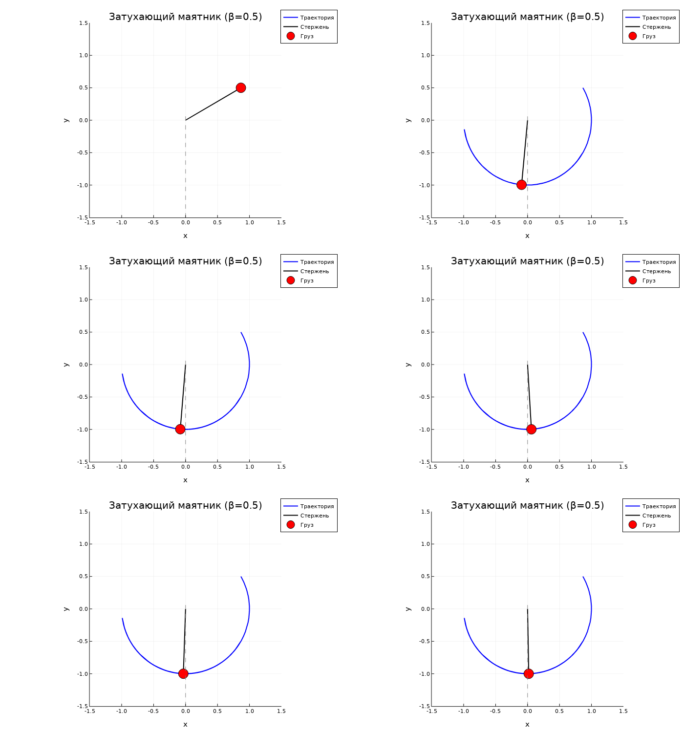
Let's move on to the model of oscillation of a mathematical pendulum without approximating small angles. In the classical problem, linearization is often used: for small deviations , which results in a simple harmonic oscillator. However, this approximation only works if rad (up to about 10-15 °). At large amplitudes (in this example The nonlinearity is significant, and the oscillation period depends on the amplitude.

The system is described by 2 first-order ODES for the angle and angular velocity :

where — attenuation coefficient. Initial conditions: , .

This example demonstrates how a numerical solution makes it possible to study systems that cannot be analytically solved, and shows the qualitative difference between nonlinear and linear oscillations.

g = 9.81
L = 1.0
β = 0.5
θ0 = deg2rad(120)
ω0 = 0.0
tspan = (0.0, 15.0)

u0 = [θ0, ω0]

function pendulum_damped!(du, u, p, t)
    du[1] = u[2]
    du[2] = -(g/L) * sin(u[1]) - β * u[2]
end

prob = ODEProblem(pendulum_damped!, u0, tspan)
sol = solve(prob, Tsit5(), saveat=0.02)

x_vals = L * sin.(sol[1,:])
y_vals = -L * cos.(sol[1,:])

@gif for i in 1:length(sol.t)
    plot(x_vals[1:i], y_vals[1:i],
         label="The trajectory", lw=2, color=:blue,
         xlabel="x", ylabel="y",
         title="Затухающий маятник (β=$β)",
         aspect_ratio=:equal,
         xlims=(-1.5, 1.5), ylims=(-1.5, 1.5))
    plot!([0, x_vals[i]], [0, y_vals[i]],
          color=:black, lw=2, label="Kernel")
    scatter!([x_vals[i]], [y_vals[i]],
             color=:red, markersize=10, label="Cargo")
    plot!([0, 0], [-1.5, 0.1],
          color=:gray, linestyle=:dash, label="")
end

Double pendulum

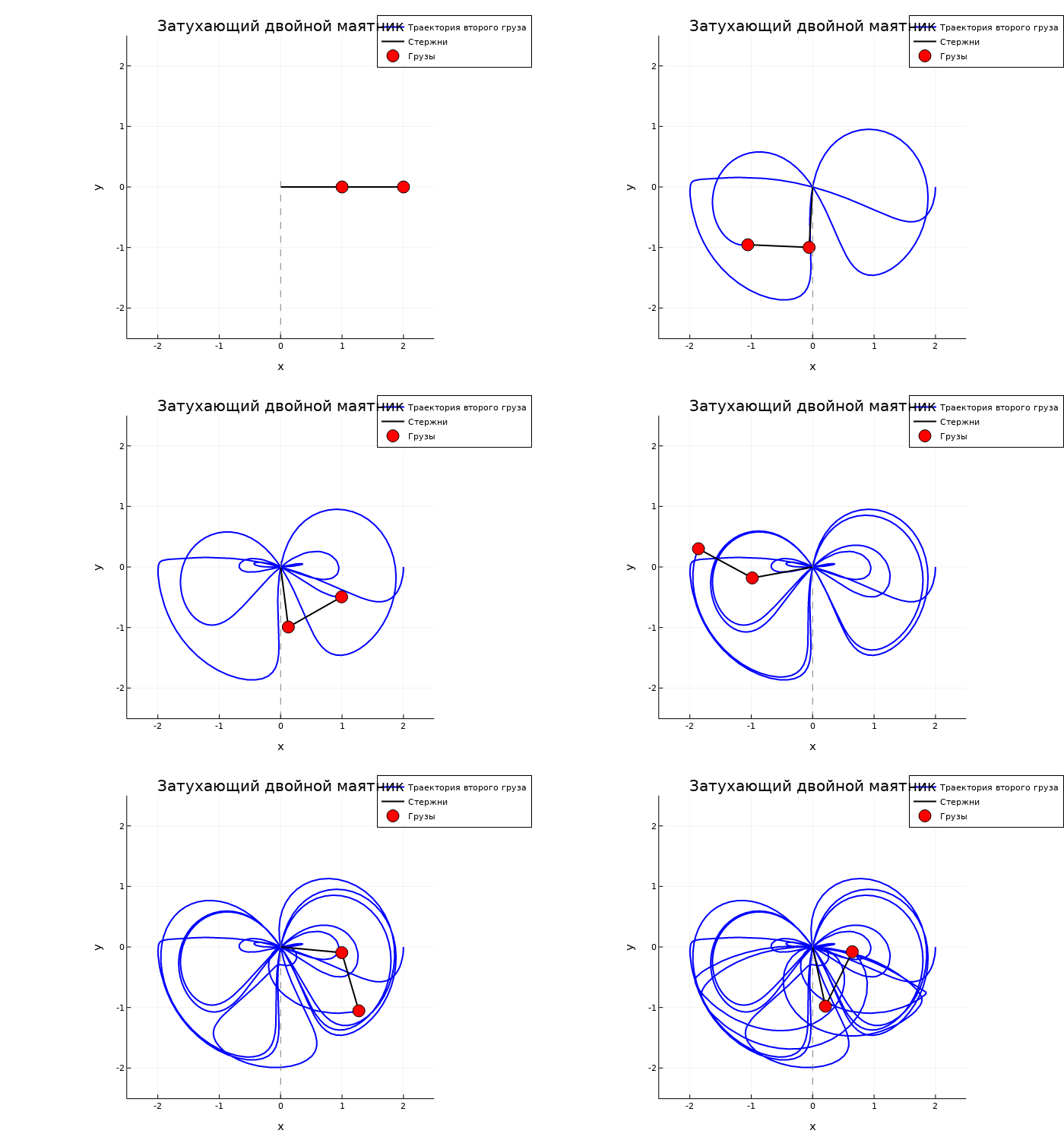
And finally, let's consider a double mathematical pendulum — two weights connected by weightless rods, oscillating in a vertical plane under the influence of gravity. This is a classic example of a chaotic system: motion is extremely sensitive to initial conditions, and the trajectory of the second load has a complex shape that is unpredictable over long periods of time. Unlike a single pendulum, there is no analytical solution here, even in the conservative case.

The system is described by 4 first-order ODES for angles and angular velocities . The equations are derived from the Lagrangian of the system and have a cumbersome appearance due to the nonlinear relationship between the links.:

where . Added attenuation coefficients in the hinges. Initial conditions: , .

This example clearly demonstrates how numerical methods make it possible to study systems for which an analytical solution is fundamentally impossible, and shows the mixing of trajectories in phase space characteristic of chaos.

L1 = L2 = 1.0
m1 = m2 = 1.0
β1 = 0.2
β2 = 0.2

θ1_0 = deg2rad(90)
θ2_0 = deg2rad(90)
ω1_0 = 0.0
ω2_0 = 0.0
u0 = [θ1_0, ω1_0, θ2_0, ω2_0]
tspan = (0.0, 15.0)

function double_pendulum_damped!(du, u, p, t)
    θ1, ω1, θ2, ω2 = u
    Δ = θ1 - θ2
    den1 = (m1 + m2) * L1 - m2 * L1 * cos(Δ)^2
    den2 = (L2 / L1) * den1

    du[1] = ω1
    du[2] = ( -g * (m1 + m2) * sin(θ1) - m2 * L1 * ω1^2 * sin(Δ) * cos(Δ)
              - m2 * g * sin(θ2) * cos(Δ) - β1 * ω1 ) / den1
    du[3] = ω2
    du[4] = ( -g * (m1 + m2) * sin(θ1) * cos(Δ)
              - (m1 + m2) * L1 * ω1^2 * sin(Δ)
              + g * (m1 + m2) * sin(θ2) - β2 * ω2 ) / den2
end

prob = ODEProblem(double_pendulum_damped!, u0, tspan)
sol = solve(prob, Tsit5(), saveat=0.02, abstol=1e-8, reltol=1e-8)

x1_vals = L1 * sin.(sol[1,:])
y1_vals = -L1 * cos.(sol[1,:])
x2_vals = x1_vals .+ L2 * sin.(sol[3,:])
y2_vals = y1_vals .- L2 * cos.(sol[3,:])

@gif for i in 1:length(sol.t)
    plot(x2_vals[1:i], y2_vals[1:i],
         label="Trajectory of the second cargo", lw=2, color=:blue,
         xlabel="x", ylabel="y",
         title="A decaying double pendulum",
         aspect_ratio=:equal,
         xlims=(-2.5, 2.5), ylims=(-2.5, 2.5))
    plot!([0, x1_vals[i], x2_vals[i]], [0, y1_vals[i], y2_vals[i]],
          color=:black, lw=2, label="Rods")
    scatter!([x1_vals[i], x2_vals[i]], [y1_vals[i], y2_vals[i]],
             color=:red, markersize=8, label="Cargo")
    plot!([0, 0], [-2.5, 0.1], color=:gray, linestyle=:dash, label="")
end

Conclusion

In this article, we have reviewed five classical mechanics problems that demonstrate the possibilities of numerical modeling in Engee using the package DifferentialEquations.jl.

Main results:

Ballistics — showed the use of an event mechanism (ContinuousCallback) to accurately determine when the condition is met (touching the ground), which is critical in many engineering tasks.
Harmonic oscillator with attenuation — demonstrated how dissipative forces qualitatively change the behavior of the system, and how, with the help of animation, one can visually observe the exponential attenuation of the amplitude.
The movement of a particle in a magnetic field — illustrated cyclotron motion and showed how the gradual drawing of the trajectory in animation helps to visualize the evolution of the system over time.
Nonlinear pendulum — demonstrated the importance of numerical methods for systems that cannot be analytically solved, and showed the qualitative difference between nonlinear and linear oscillations at large amplitudes.
Double pendulum — presented a classic example of a chaotic system where the trajectory is extremely sensitive to initial conditions, and showed the need for high accuracy tolerances (abstol=1e-8, reltol=1e-8) for the correct modeling of such systems.